The journey to today's version of QuestDB began with the original prototype in 2013, and we've described what happened since in a post published during our HN launch last year. In the early stages of the project, we were inspired by vector-based append-only systems like kdb+ because of the advantages of speed and the simple code path this model brings. We also required that row timestamps were stored in ascending order, resulting in fast time series queries without an expensive index.
We found out that this model does not fit all data acquisition use cases, such as out-of-order data. Although several workarounds were available, we wanted to provide this functionality without losing the performance we spent years building.
We studied existing approaches, and most came at a performance cost that we weren't happy with. Like the entirety of our codebase, the solution that we present today is built from scratch. It took over 9 months to come to fruition and adds a further 65k lines of code to the project.
Here's what we built, why we built it, what we learned along the way, and benchmarks comparing QuestDB to InfluxDB, ClickHouse and TimescaleDB.
The problem with out-of-order data
Our data model had one fatal flaw - records were discarded if they appear out-of-order (O3) by timestamp compared to existing data. In real-world applications, payload data doesn’t behave like this because of network jitter, latency, or clock synchronization issues.
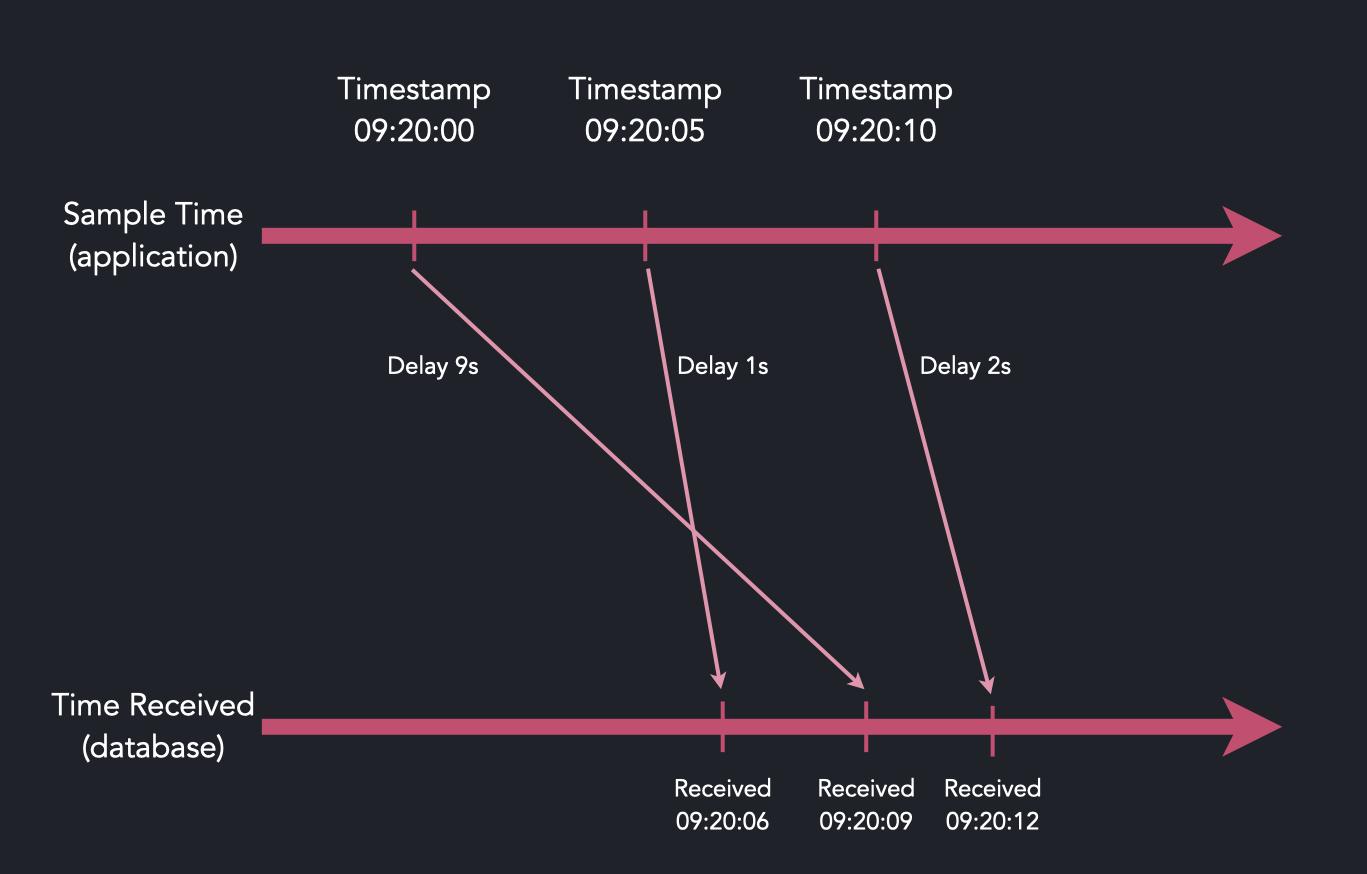
We knew that the lack of out-of-order support was a show-stopper for some users and we needed a solid solution. There were possible workarounds, such as using a single table per data source or re-ordering tables periodically, but for most users this is inconvenient and unsustainable.
How should you store out-of-order time series data?
As we reviewed our data model, one possibility was to use something radically different from what we already had, such as including LSM trees or B-trees, commonly used in time series databases. Adding trees would bring the benefit of being able to order data on the fly without inventing a replacement storage model from scratch.
What bothered us most with this approach is that every subsequent read operation would face a performance penalty versus having data stored in arrays. We would also introduce complexity by having a storage model for ordered data and another for out-of-order data.
A more promising option was to introduce a sort-and-merge phase as data arrives. This way, we could keep our storage model unchanged, while merging data on the fly, with ordered vectors landing on disk as the output.
Early thoughts on a solution
Our idea of how we could handle out-of-order ingestion was to add a three-stage approach:
- Keep the append model until records arrive out-of-order
- Sort uncommitted records in a staging area in-memory
- Reconcile and merge the sorted data and persisted data at commit time
The first two steps are straightforward and easy to implement, and handling append-only data is unchanged. The heavy commit kicks in only when there is data in the staging area. The bonus of this design is that the output is vectors, meaning our vector-based readers are still compatible.
This pre-commit sort-and-merge adds an extra processing phase to ingestion with an accompanying performance penalty. We nevertheless decided to explore this approach and see how far we could reduce the penalty by optimizing the heavy commit.
How we sort, merge, and commit out-of-order time series data
Processing a staging area in bulk gives us a unique opportunity to analyze the
data holistically. Such analysis aims to avoid physical merges altogether
where possible and perhaps get away with fast and straightforward memcpy or
similar data movement methods. Such methods can be parallelized thanks to our
column-based storage. We can employ SIMD and non-temporal data access where it
makes a difference.
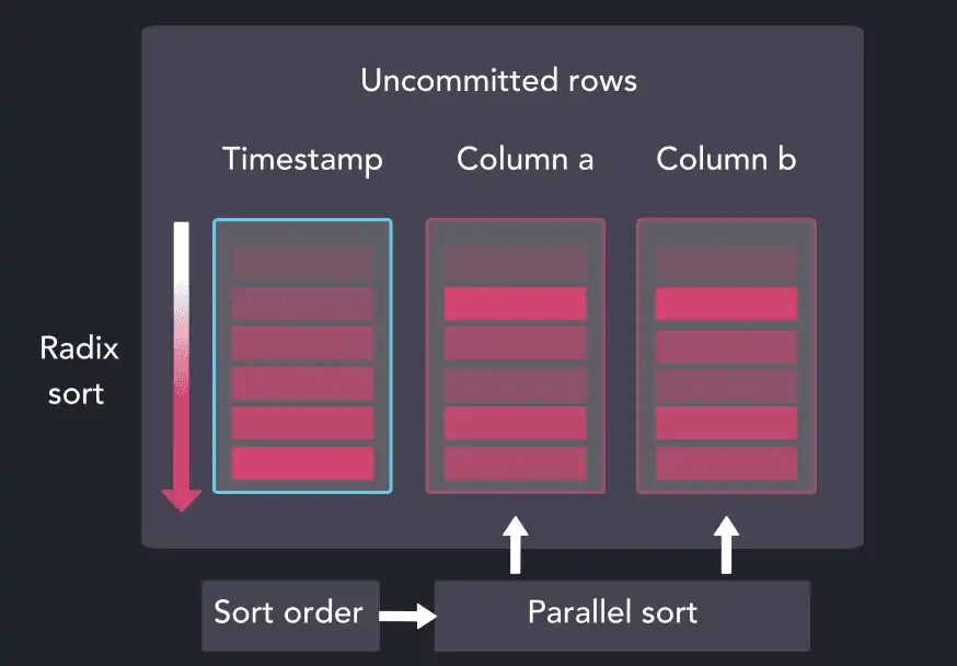
We sort the timestamp column from the staging area via an optimized version of radix sort, and the resulting index is used to reshuffle the remaining columns in the staging area in parallel:
The now-sorted staging area is mapped relative to the existing partition data. It may not be obvious from the start but we are trying to establish the type of operation needed and the dimensions of each of the three groups below:
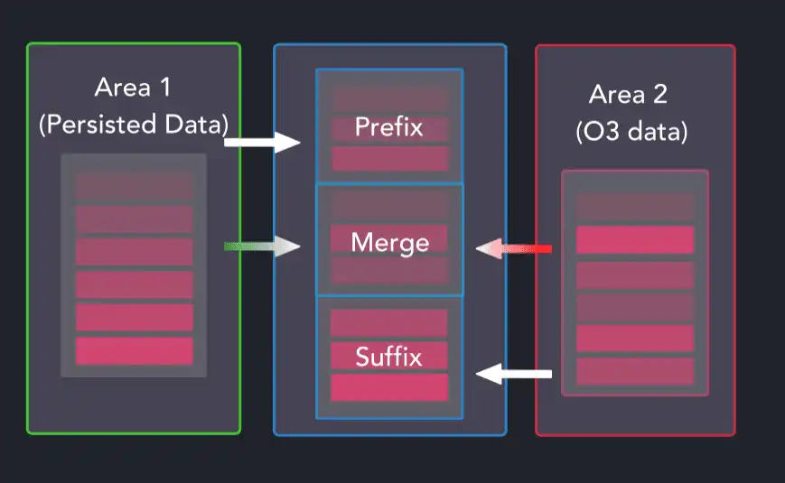
When merging datasets in this way, the prefix and suffix groups can be persisted data, out-of-order data, or none. The merge group is where more cases occur as it can be occupied by persisted data, out-of-order data, both out-of-order and persisted data, or none.
When it's clear how to group and treat data in the staging area, a pool of
workers perform the required operations, calling memcpy in trivial cases and
shifting to SIMD-optimized code for everything else. With a prefix, merge, and
suffix split, the maximum liveliness of the commit (how susceptible it is to
add more CPU capacity) is partitions_affected x number_of_columns x 3.
Optimizing copy operations with SIMD
Because we aim to rely on memcpy the most, we benchmarked code that merges
variable-length columns:
template<typename T>
inline void merge_copy_var_column(
        index_t *merge_index,
        int64_t merge_index_size,
        int64_t *src_data_fix,
        char *src_data_var,
        int64_t *src_ooo_fix,
        char *src_ooo_var,
        int64_t *dst_fix,
        char *dst_var,
        int64_t dst_var_offset,
        T mult
) {
    int64_t *src_fix[] = {src_ooo_fix, src_data_fix};
    char *src_var[] = {src_ooo_var, src_data_var};

    for (int64_t l = 0; l < merge_index_size; l++) {
        MM_PREFETCH_T0(merge_index + l + 64);
        dst_fix[l] = dst_var_offset;
        const uint64_t row = merge_index[l].i;
        const uint32_t bit = (row >> 63);
        const uint64_t rr = row & ~(1ull << 63);
        const int64_t offset = src_fix[bit][rr];
        char *src_var_ptr = src_var[bit] + offset;
        auto len = *reinterpret_cast<T *>(src_var_ptr);
        auto char_count = len > 0 ? len * mult : 0;
        reinterpret_cast<T *>(dst_var + dst_var_offset)[0] = len;
        __MEMCPY(dst_var + dst_var_offset + sizeof(T), src_var_ptr + sizeof(T), char_count);
        dst_var_offset += char_count + sizeof(T);
    }
}
with __MEMCPY as Angner Fog's Asmlib A_memcpy, in one instance and glibC's
memcpy in the other.
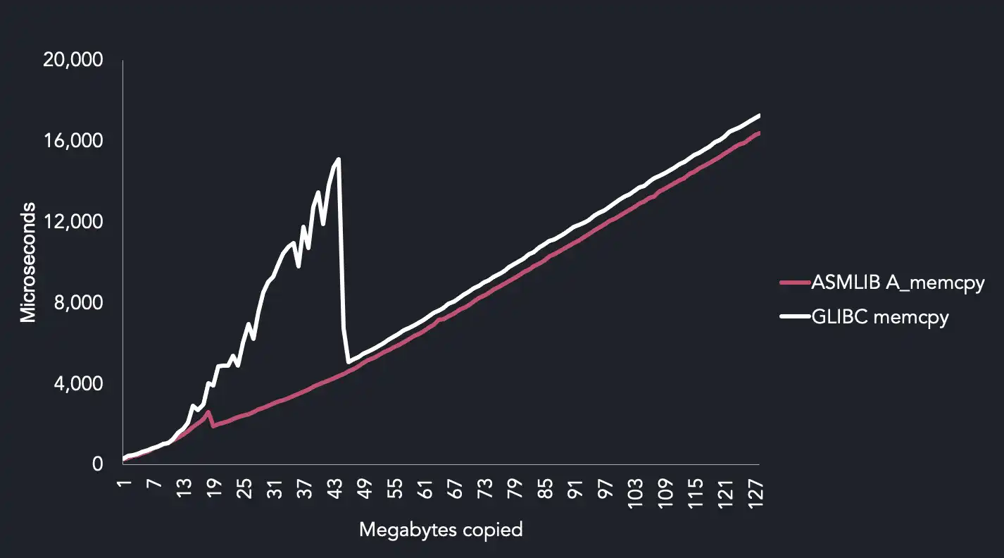
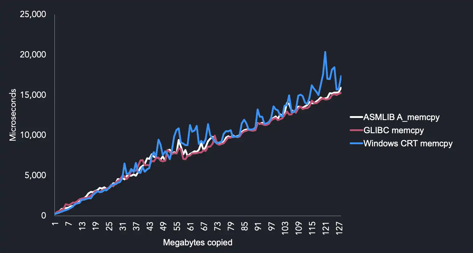
The key results from this comparison are:
glibccould be slow and inconsistent on AVX512 for our use case. We speculate thatA_memcpydoes better because it uses non-temporal copy instructions.- Windows
memcpyis pretty bad. A_memcpyandmemcpyperform well on CPUs below AVX512.
A_memcpy uses non-temporal streaming instruction which appear to work well
with the following simple loop:
template<typename T>
void set_memory_vanilla(T *addr, const T value, const int64_t count) {
   for (int64_t i = 0; i < count; i++) {
       addr[i] = value;
   }
}
The above is a memory buffer filled with the same 64 bit pattern. It can be
implemented as memset if all bytes are the same. It also can be written as
vectorized code which uses platform-specific _mm??_stream_ps(p,?mm) in
store_nt vector method, as seen below:
template<typename T, typename TVec>
inline void set_memory_vanilla(T *addr, const T value, const int64_t count) {

    const auto l_iteration = [addr, value](int64_t i) {
        addr[i] = value;
    };

    const TVec vec(value);
    const auto l_bulk = [&vec, addr](const int64_t i) {
        vec.store_nt(addr + i);
    };

    run_vec_bulk<T, TVec>(addr, count, l_iteration, l_bulk);
}
The results were quite surprising. Non-temp SIMD instructions showed the most
stable results with similar performance to memset.
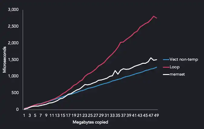
Unfortunately, benchmark results with other functions were less conclusive. Some perform better with hand-written SIMD and some just as fast with GCC's SSE4 generated code even when it is ran on AVX512 systems.
Hand-writing SIMD instructions is both time consuming and verbose. We ended up optimizing parts of the code base with SIMD only when the performance benefits outweighed code maintenance.
How often should data be ordered and merged?
While being able to copy data fast is a good option, we think that heavy data copying can be avoided in most time series ingestion scenarios. Assuming that most real-time out-of-order situations are caused by the delivery mechanism and hardware jitter, we can deduce that the timestamp distribution will be locally contained by some boundary.
For example, if any new timestamp value has a high probability to fall within 10 seconds of the previously received value, the boundary is then 10 seconds, and we call this boundary lag.
When timestamp values follow this pattern, deferring the commit can render out-of-order commits a normal append operation. The out-of-order system can deal with any variety of lateness, but if incoming data is late within the time specified as lag, it will be prioritized for faster processing.
Comparing ingestion with ClickHouse, InfluxDB and TimescaleDB
We saw the Time Series Benchmark Suite (TSBS) regularly coming up in discussions about database performance and decided we should provide the ability to benchmark QuestDB along with other systems.
The TSBS is a collection of Go programs to generate datasets and then benchmark read and write performance. The suite is extensible so that different use cases and query types can be included and compared across systems.
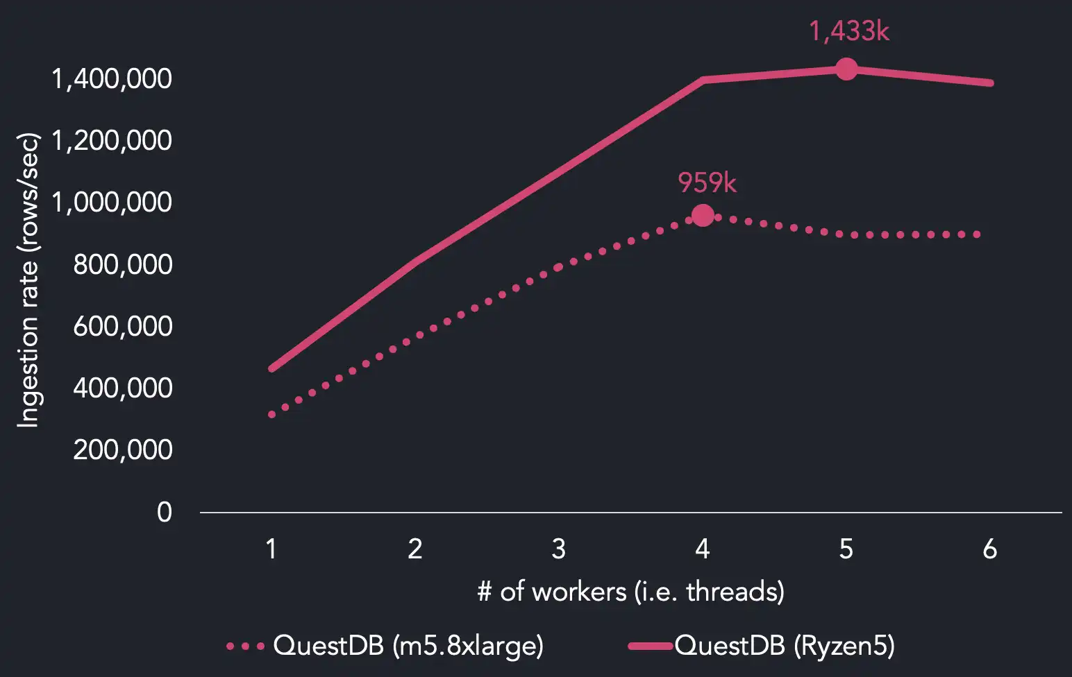
Here are our results of the benchmark with the cpu-only use case using up to
fourteen workers on an AWS EC2 m5.8xlarge instance with sixteen cores.
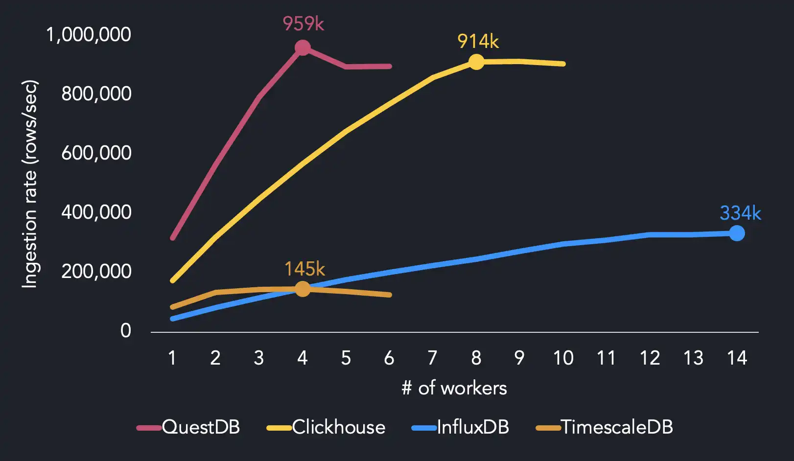
We reach maximum ingestion performance using four threads, whereas the other systems require more CPU resources to hit maximum throughput. QuestDB achieves 959k rows/sec with 4 threads. We find that InfluxDB needs 14 threads to reach its max ingestion rate (334k rows/sec), while TimescaleDB reaches 145k rows/sec with 4 threads. ClickHouse hits 914k rows/sec with twice as many threads as QuestDB.
When running on 4 threads, QuestDB is 1.7x faster than ClickHouse, 6.4x faster than InfluxDB and 6.5x faster than TimescaleDB.
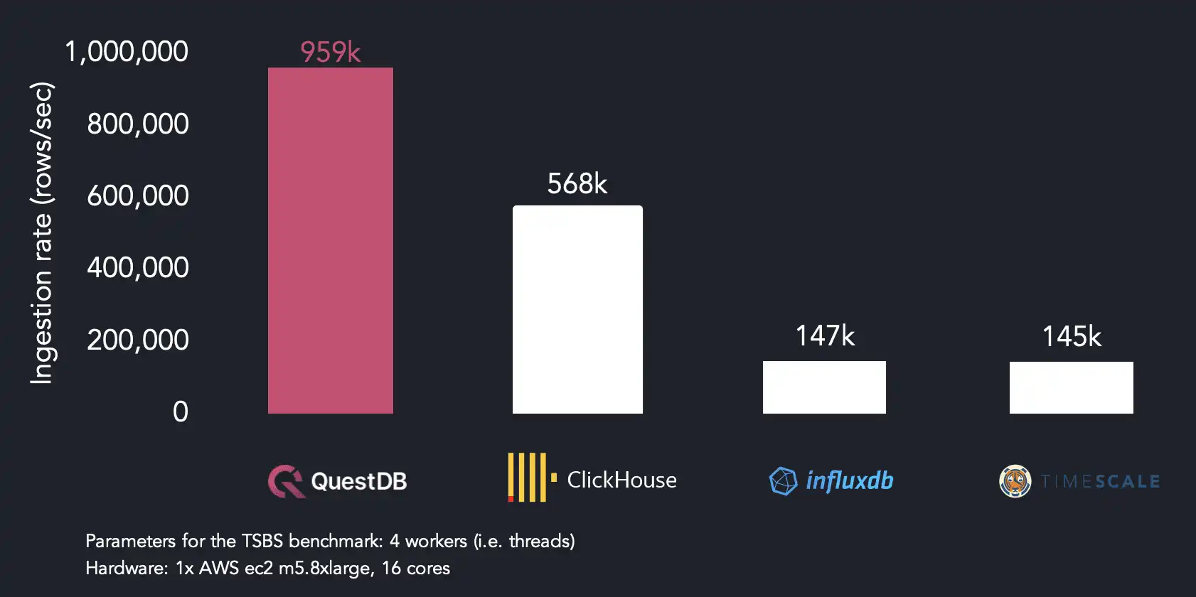
Because our ingestion format (ILP) repeats tag values per row, ClickHouse and TimescaleDB parse around two-thirds of the total volume of data as QuestDB does in the same benchmark run. We chose to stick with ILP because of its widespread use in time series, but we may use a more efficient format to improve ingestion performance in the future.
Finally, degraded performance beyond 4 workers can be explained by the increased contention beyond what the system is capable of. We think that one limiting factor may be that we are IO bound as we scale up to 30% better on faster AMD-based systems.
When we run the suite again using an AMD Ryzen5 processor, we found that we were
able to hit maximum throughput of 1.43 million rows per second using 5 threads.
This is compared to the
Intel Xeon Platinum that's in use
by our reference benchmark m5.8xlarge instance on AWS.
Adding QuestDB support to the Time Series Benchmark Suite
We have opened a pull request (#157 - Questdb benchmark support) in TimescaleDB's TSBS GitHub repository which adds the ability to run the benchmark against QuestDB. In the meantime, readers may clone our fork of the benchmark suite and run the tests to see the results for themselves.
# Generating the dataset
tsbs_generate_data --use-case="cpu-only" --seed=123 --scale=4000 \
  --timestamp-start="2016-01-01T00:00:00Z" \
  --timestamp-end="2016-01-02T00:00:00Z" \
  --log-interval="10s" --format="influx" > /tmp/bigcpu
# Loading the data
tsbs_load_questdb --file /tmp/bigcpu --workers 4
To add out-of-order support, we went for a novel solution that yielded surprisingly good performance versus well-trodden approaches such as B-trees or LSM-based ingestion frameworks. We're happy to have shared the journey, and we're eagerly awaiting feedback from the community.
For more details, the GitHub release for version 6.0 contains a changelog of additions and fixes in this release.