A few months back I was working on the primary-replica replication feature in QuestDB. The feature was nearing completion of development but we had a report that it was using a significant amounts of network bandwidth.
During the process of debugging the issue I ended up implementing my own quick'n'dirty network profiling tooling. This is a blog post on how I wrote the tool and how I analysed the data.
The performance problem
A bit of context first: Our database instances do not replicate directly point-to-point. Instead, they compress and upload the table's WAL (write-ahead log) files to a central object store such as AWS S3 or Azure Blob store. In other words, we store each table's full edit history in a series of files in the object store that we can replay back at any time.
This architecture:
- decouples deployment
- allows rebuilding a database instance up to a specific transaction point
- is generally more scalable
By delegating the work to an external component, it relieves the primary database instance from having to deal with serving the replica instances.
Each uploaded file (segment) contains a block of transactions. We overwrite the last file over and over with more transactions until it's large enough to roll over to the next file. We need to do this because the compatible object stores we use, for the most part, do not support appending.
Being a time series database, users would typically stream (ingest) records into the database at a relatively constant rate (consuming network bandwidth inbound). The primary database instance would then write artifacts to the object store (consuming network bandwidth outbound).
On an early deployment on DigitalOcean, we noticed that our outbound object store bandwidth usage was significantly higher than the inbound ingestion bandwith usage. Not only that, but the outbound object store bandwidth usage kept growing hour by hour. And it did so despite a constant ingestion rate.
I've lost the original metrics and numbers, but it would have looked something like the following diagram (use your imagination to imagine the usual network bandwidth usage noise):

Needless to say that the replication bandwidth should be roughly proportional to the ingestion bandwidth and not grow over time!
Capturing the network traffic
I needed to understand what was going on accurately, so at first I turned to Wireshark. I hoped I could perform a simulated test run and capture a time series about packet sizes for both the inbound and outbound connections, but struggled to do this. It's likely possible to accomplish this in Wireshark, but I find its UI pretty daunting, and I'm more comfortable with writing code.
Wireshark is built on packet capture, so instead I grabbed my favourite tool
(Rust) and used the pcap crate (wrapping the
libpcap C library) to capture the two time series.
For each connection, whenever I'd observe a packet I'd capture two fields:
- The packet's timestamp (
i64epoch nanos timestamp). - The packet's size (
u64).
After writing a script to generate some load, I set up my test with
s3s-fs - a binary that emulates an AWS S3
endpoint, then ran a primary QuestDB instance on the same machine.
I could now monitor the database's inbound traffic on port 9000 and the
replication traffic on port 10101 using a net-traffic-capture tool I I wrote
for this purpose in Rust.
Here are the first few lines of the main function of the packet capture tool.
They run a loop over the intercepted traffic for the specific ports over the
loopback device.
For the full code see github.com/questdb/replication-stats -> /net-traffic-capture/.
fn main() -> anyhow::Result<()> {
    // ...
    let ports: HashSet<_> = ports.into_iter().collect();
    let writer_queue = writer::Writer::run(dir);
    let device = get_loopback_device()?;
    let mut cap = Capture::from_device(device)?
        .promisc(false)
        .snaplen(128)
        .timeout(1)
        .buffer_size(4 * 1024 * 1024)
        .open()?;
    cap.filter("tcp", true)?;
    let link_type = cap.get_datalink();
    loop {
        let packet = ignore_timeouts(cap.next_packet())?;
        let Some(packet) = packet else {
            continue;
        };
        let tcp_data = parse_tcp(&packet, link_type)?;
        let Some(tcp_data) = tcp_data else {
            continue;
        };
        // ...
    }
}
The byte parsing logic here is implemented using the excellent
etherparse crate.
fn parse_tcp(
    packet: &Packet,
    link_type: Linktype
) -> anyhow::Result<Option<TcpData>> {
    if packet.header.caplen < 32 {
        return Ok(None);
    }
    let ipv4data = match link_type {
        Linktype::NULL => &packet.data[4..],
        Linktype::ETHERNET => skip_ethernet_header(packet.data)?,
        _ => return Err(anyhow::anyhow!(
            "Unsupported link type: {:?}", link_type)),
    };
    let sliced = SlicedPacket::from_ip(ipv4data)?;
    let Some(InternetSlice::Ipv4(ipv4slice, _)) = sliced.ip else {
        return Ok(None);
    };
    let src_addr = ipv4slice.source_addr();
    let dest_addr = ipv4slice.destination_addr();
    let TransportSlice::Tcp(tcp) = sliced.transport.unwrap() else {
        return Ok(None);
    };
    let src_port = tcp.source_port();
    let dest_port = tcp.destination_port();

    let link_bytes_len = 4;
    let data_offset = link_bytes_len +
        ((ipv4slice.ihl() * 4) + (tcp.data_offset() * 4)) as usize;
    let tcp_data = TcpData {
        ts: to_system_time(packet.header.ts),
        src: Addr {
            ip: src_addr,
            port: src_port,
        },
        dest: Addr {
            ip: dest_addr,
            port: dest_port,
        },
        data_offset,
        flags: TcpMeta::from_tcp_header(&tcp),
    };
    Ok(Some(tcp_data))
}
Once parsed, I had to write these time series metrics to disk in a format I could analyse easily later.
Being a database engineer, I've got this: I re-implemented a tiny subset of QuestDB's ingestion logic in Rust. One thread sits on the pcap loop listening and parsing network packets, passing messages over a message queue to another thread responsible to append the time series to disk.
I could have captured the data into another QuestDB instance, but I was concerned that this might skew the results.
The thread that's responsible for disk writing uses growable memory mapped files to write the data into a columnar format. In other words, for each of the two time series, there's a timestamp column and a packet size column.
// writer.rs
struct U64ColWriter {
    file: std::fs::File,
    mmap: MmapMut,
    len: u64,
    cap: u64,
}

impl U64ColWriter {
    fn new(path: &Path) -> io::Result<Self> {
        let cap = increment();
        let file = std::fs::OpenOptions::new()
            .read(true)
            .write(true)
            .create(true)
            .truncate(true)
            .open(path)
            .unwrap();
        file.set_len(cap)?;
        let mmap = unsafe { MmapMut::map_mut(&file)? };
        Ok(Self {
            file,
            mmap,
            len: 0,
            cap,
        })
    }

    fn may_resize(&mut self) -> io::Result<()> {
        let required = self.len + size_of::<u64>() as u64;
        if required < self.cap {
            return Ok(());
        }
        self.cap += increment();
        self.file.set_len(self.cap)?;
        self.mmap = unsafe { MmapMut::map_mut(&self.file)? };
        Ok(())
    }

    fn append(&mut self, val: u64) -> io::Result<()> {
        self.may_resize()?;
        let offset = self.len as usize;
        self.mmap[offset..offset + size_of::<u64>()]
            .copy_from_slice(&val.to_le_bytes());
        self.len += size_of::<u64>() as u64;
        Ok(())
    }
}
All we need now is to add an extra .count file to track the number of written
rows. The code updates it last after writing the two column files.
impl DatapointWriter {
    fn new(path: &Path) -> io::Result<Self> {
        let ts_writer = U64ColWriter::new(
            &path.with_extension("ts"))?;
        let val_writer = U64ColWriter::new(
            &path.with_extension("val"))?;
        let count_writer = CountWriter::new(
            &path.with_extension("count"))?;
        Ok(Self {
            ts_writer,
            val_writer,
            count_writer,
        })
    }

    fn append(&mut self, ts: u64, val: u64) -> io::Result<()> {
        self.ts_writer.append(ts)?;
        self.val_writer.append(val)?;
        self.count_writer.increment()
    }
}
Memory mapped files reduce the number of system calls and also allow the kernel to decide when to flush the data to disk in a very efficient manner. What's more, once written to memory, the data is safe within the kernel and can survive a process crash (but not a kernel panic or a sudden power cut). This makes it "transactional enough" for most use cases, and certainly for this one. The reason for using two threads is that writing to memory mapped files is still a blocking IO operation and I did not want to slow down the pcap loop.
Analysing the network traffic
Now over to my second favourite tool: Python. The column files written are
effectively just packed 64-bit integers. A few lines of pyarrow later and the
collected samples are loaded into a pyarrow.Table and from that, loaded
zero-copy into a polars.DataFrame.
For the full code see github.com/questdb/replication-stats -> /analisys/.
# analisys/reader.py
def read_col(count, dtype, path):
    with open(path, 'rb') as col_file:
        mem = mmap.mmap(
            col_file.fileno(),
            length=count * 8,
            access=mmap.ACCESS_READ)
        buf = pa.py_buffer(mem)
        return pa.Array.from_buffers(dtype, count, [None, buf])

def read_port_table(port, name, data_dir):
    data_dir = Path(data_dir)
    with open(data_dir / f'{port}.count', 'rb') as f:
        count = struct.unpack('<Q', f.read())[0]
    ts_arr = read_col(
        count, pa.timestamp('ns'), data_dir / f'{port}.ts')
    val_arr = read_col(
        count, pa.uint64(), data_dir / f'{port}.val')
    return pl.from_arrow(
        pa.Table.from_arrays(
            [ts_arr, val_arr], names=['ts', name])
    ).sort('ts')
At this stage I was ready to launch Jupyter Lab and start dissecting the table and plot some graphs!
When I originally ran my simulation, I did so in a way that simulated time 100x faster than real time. The code below loads it and scales the timestamps back to real time.
data = read_ports_table(
    {9000: 'ilp', 10101: 'replication'},
    data_dir='../captures/' + data_dir,
    scale_ts=scaling)
The data is now merged into a single table with a single ts timestamp column
(ordered) and two packet size columns, one for each port. These two are labelled
ilp (for ingestion) and replication (for the mock AWS S3 traffic).
In this sample data you'll notice one of the columns is zero. This is because that port had no traffic at that timestamp.
| ts : datetime[ns] | ilp : u64 | replication : u64 |
|---|---|---|
| 2024-02-06 17:50:31.517389 | 0 | 376 |
| 2024-02-06 17:50:31.709789 | 0 | 414 |
| 2024-02-06 17:50:32.311689 | 0 | 649 |
| 2024-02-06 17:50:32.349789 | 0 | 669 |
| 2024-02-06 17:50:32.402989 | 0 | 677 |
| 2024-02-06 17:50:33.045389 | 0 | 459 |
| 2024-02-06 17:50:33.360989 | 0 | 699 |
| 2024-02-06 17:50:33.363089 | 0 | 667 |
| 2024-02-06 17:50:33.370589 | 0 | 690 |
| 2024-02-06 17:50:35.635789 | 0 | 500 |
| 2024-02-06 17:50:36.178789 | 0 | 546 |
| 2024-02-06 17:50:36.318489 | 0 | 593 |
| … | … | … |
The next task is to group by time: Individual packet sizes and timestamps are not useful. We need a bandwidth usage metric in bytes/sec over a sampling interval.
If I had loaded the data into QuestDB, I'd now be able to use the SAMPLE BY
SQL statement. In Polars we can use the group_by_dynamic function.
grouping_window = 60 * 1000  # millis
scale = 1000 / grouping_window
grouped = data.group_by_dynamic(
    "ts",
    every=f"{grouping_window}ms"
    ).agg(
        pl.col("ilp").sum() * scale,
        pl.col("replication").sum() * scale)
grouped
The grouped table now contains the bandwidth usage for each port over a
sampling interval.
| ts : datetime[ns] | ilp : f64 | replication : f64 |
|---|---|---|
| 2024-02-06 17:50:00 | 0.0 | 137.783333 |
| 2024-02-06 17:57:00 | 104.433333 | 23.683333 |
| 2024-02-06 17:58:00 | 433.8 | 124.166667 |
| 2024-02-06 17:59:00 | 417.733333 | 143.066667 |
| 2024-02-06 18:00:00 | 425.766667 | 160.883333 |
| 2024-02-06 18:01:00 | 433.8 | 182.566667 |
| 2024-02-06 18:02:00 | 449.866667 | 204.5 |
| 2024-02-06 18:03:00 | 441.833333 | 225.25 |
| 2024-02-06 18:04:00 | 449.866667 | 245.8 |
| 2024-02-06 18:05:00 | 441.833333 | 303.566667 |
| 2024-02-06 18:06:00 | 425.766667 | 91.633333 |
| 2024-02-06 18:07:00 | 409.7 | 158.333333 |
| … | … | … |
Plottable data, finally.
import plotly.express as px
fig = px.line(
    grouped,
    x='ts',
    y=['ilp', 'replication'],
    markers=False,
    line_shape='hv',
    labels={'ts': 'timestamp', 'value': 'bytes/sec'},
    template='plotly_dark')
fig.show()
This tooling allowed me to quickly identify the problem. It turns out that we
were re-uploading the full table's transaction metadata from the start (i.e.
from CREATE TABLE onwards).
The fix was to instead distribute the table metadata across multiple files so it can be uploaded incrementally without causing network usage growth.
With the fix in place I was then able to use this network analysis tooling to further fine tune the replication algorith such that replicating between instances is now more bandwidth efficient than ingestion itself.
This same tooling also helped me build the replication tuning guide for QuestDB.
This is one of the final plots generated by the tool running replication with network-bandwidth optimized parameters.
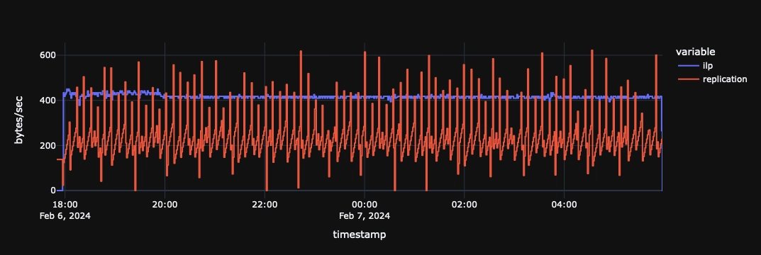
The value of the tool is clearer when zooming into a particular section of the plot.
In the plot below it's pretty easy to spot the zig-zag pattern caused by continuously re-uploading the last active segment, with a fall-off once the segment is rolled over.

Summary
This blog post shows a basic approach for programmatic packet capture and how it's then easy to plot the captured time series metrics in Python and Polars.
You also had a chance to see the techniques we use inside QuestDB itself to obtain great ingestion performance.
Come talk to us on Slack or Discourse!