Tracking sea faring ships with AIS data and Grafana

# Drunken Sailor - Ye' old sea shanty
What shall we do with a drunken sailor?
What shall we do with a drunken sailor?
What shall we do with a drunken sailor?
Early in the morning!

What shall we do? We'd keep an eye on their boat, that's for sure. Who knows where it could wind up? In this post, we will look at historical location data from the Automatic Identification System (AIS) to analyze traffic and create visualizations to have us chart the ships that sail the seas.

There will be no more singing. Weigh the anchor! Hoist the sails! Make way!

What is the Automatic Identification System?​

The Automatic Identification System broadcasts ship data. It works by leveraging the ships' onboard transceivers which communicate their position, course, speed, and other metrics. It is mostly intended as an anti-collision system to support traffic controllers and coast guards in addition to other means such as radar.

For certain ship sizes, continuous AIS data transmission is often a regulatory requirement. As a result, the AIS transceivers are typically always on. Turning the AIS system off may in some cases indicate that a ship is attempting to hide their position, possibly to hide illegal activity such as off-radar fishing or sanctions evasion such as North Korea oil smuggling. And that can attract the attention of authorities.

Typical AIS data would include:

• the ship's position
• bearing
• speed
• type
• a unique identifier called MMSI, the Maritime Mobile Service Identity
• journey start and end time

If this sounds like "time-series data", you're correct. This data exemplifies the burst-y, high-volume and highly sensitive nature of time-series data. And so to power our analysis we can use a specialized time-series database like QuestDB.

Ingesting AIS data​

The Marine Cadastre offers historical data of tracked ships within the United States region. While this data is not realtime, it is still useful to take a look at traffic around the US.

To use the data, we first download one of the archives from the Marine Cadastre and then extract it. The result is a SQLite database comprising a few tables.

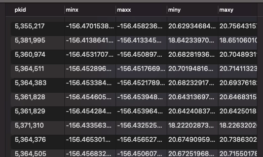
The table st_spindex\_\_AISVesselTracks2022_Shape lists coordinates in latitude (y) and longitude (x). It shows two coordinate sets:

1. minX and minY which act as the starting latitudes/longitudes
2. maxY,maxY which act as the ending coordinates

The pkid column seems to be a key to lookup the ship against another table:

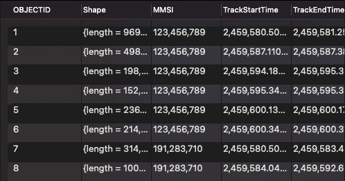
The table AISVesselTracks2022 contains an objectID which is again a primary key, alongside the MMSI identification numbers, the TrackStartTime and the TrackEndTime which are timestamp measures:

There are other tables in the dataset which seem to contain some geometry and are apparently intended to be used with specialized AIS analysis software. While we do not have such software, we can make assumptions as we interpret the data.

Our first assumption was that minX/minY are starting coordinates and that maxX/maxY are ending coordinates. The second assumption has to do with timestamps, and how they may relate to our first assumption.

Parsing timestamps​

To begin, import the above two tables into QuestDB as CSV files. But when we do, the timestamps look curious. The data above relates to 2022, so it's natural that we would assume that the timestamps are distributed between 01-Jan-2022 and 31-Dec-2022. However, the timestamps don't appear as normal unix epochs. And there is no documentation explaining them:

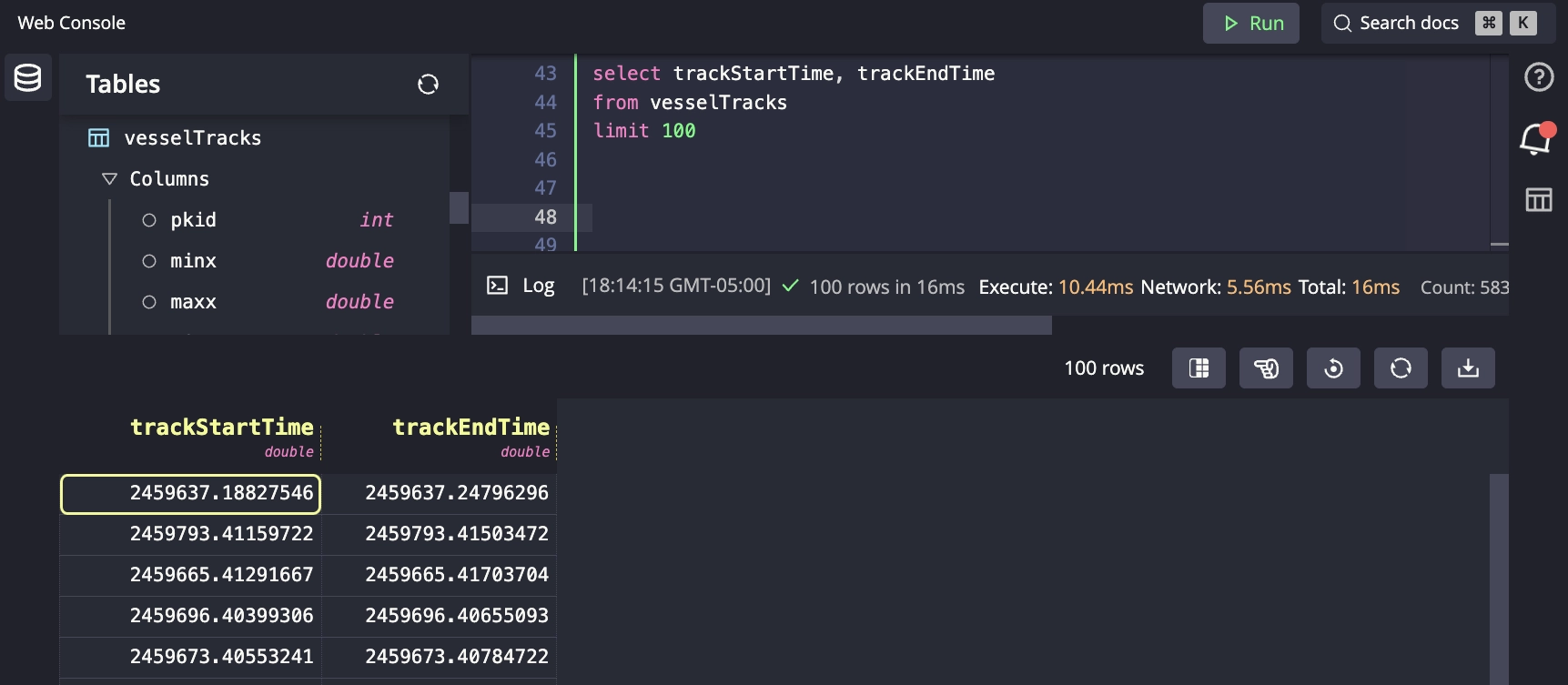
First, the timestamps include decimal fractions. For example 2459637.18827546.

Second, they don't appear to be multiples of epochs. For example, the epoch for January 1, 2022, was 1704067201 in seconds.

We also tried various approaches such as multiplying by factors of 60, 24, 1000, 10000 and combinations thereof but could not generate any meaningful timestamp.

What else can we try? Hmm...

SELECT
    max(trackEndTime) - min(trackStartTime)
FROM
    vesselTracks

# Returns
>> 364.999988430179

The result of the above is 364.999988430179 which seems to suggest that the integer part of the timestamp represents one day, and the decimal part a fraction of days.

Let's infer that the first value is very close to midnight on the 1st of Jan 2022:

SELECT min(trackStartTime)
FROM vesselTracks
>> 2459580.5

With this anchor point, we can calculate an offset from the 1st of Jan 2022 to get an approximate timestamp by adding an offset in seconds:

SELECT
    dateadd(
        's',
        cast((trackEndTime - 2459580.0) * 24 * 60 * 60 as int),
        to_timestamp('2022-01-01', 'yyyy-MM-dd')
    )
FROM
    vesselTracks

# Returns...
trackStartTime	timestamp
2459637.18827546	2022-02-26T16:31:06.000000Z
2459793.41159722	2022-08-01T21:52:41.000000Z
2459665.41291667	2022-03-26T21:54:36.000000Z
2459696.40399306	2022-04-26T21:41:45.000000Z
2459673.40553241	2022-04-03T21:43:58.000000Z
2459662.25149306	2022-03-23T18:02:09.000000Z

Creating a new time-series​

We assumed that the min and max coordinates correspond to the timestamps trackStartTime and trackEndTime. From there, we can use a SQL UNION to create a new table with a unique timestamp column. We can create two rows for each entry, for the starting and ending positions respectively.

We can also leverage ORDER BY timestamp ASC and timestamp(timestamp) to create the designated ordered timestamp column:

CREATE TABLE vessels AS
(
  (
    SELECT MMSI,trackStartTime,
            dateadd('s',cast((trackStartTime-2459580.5)*24*60*60 as int),
                    to_timestamp('2022-01-01','yyyy-MM-dd')) timestamp,
            minX longitude, minY latitude,
            cast(vesselGroup AS symbol) vesselGroup,
            Length, Width, Draft
    FROM vesselTracks
UNION
    SELECT MMSI,trackEndTime,
            dateadd('s',cast((trackEndTime-2459580.5)*24*60*60 as int),
                    to_timestamp('2022-01-01','yyyy-MM-dd')) timestamp,
            maxX longitude, maxY latitude,
            cast(vesselGroup AS symbol) vesselGroup,
            Length, Width, Draft
    FROM vesselTracks
  )
  ORDER BY timestamp ASC
) timestamp(timestamp)

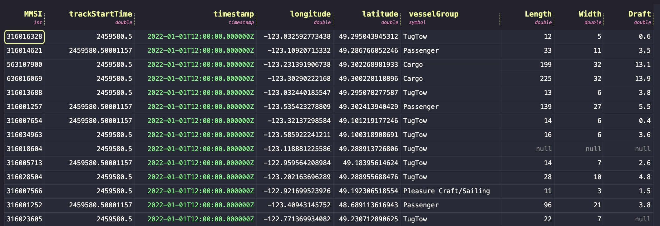
Our table looks like this:

Tracking ships with a heatmap​

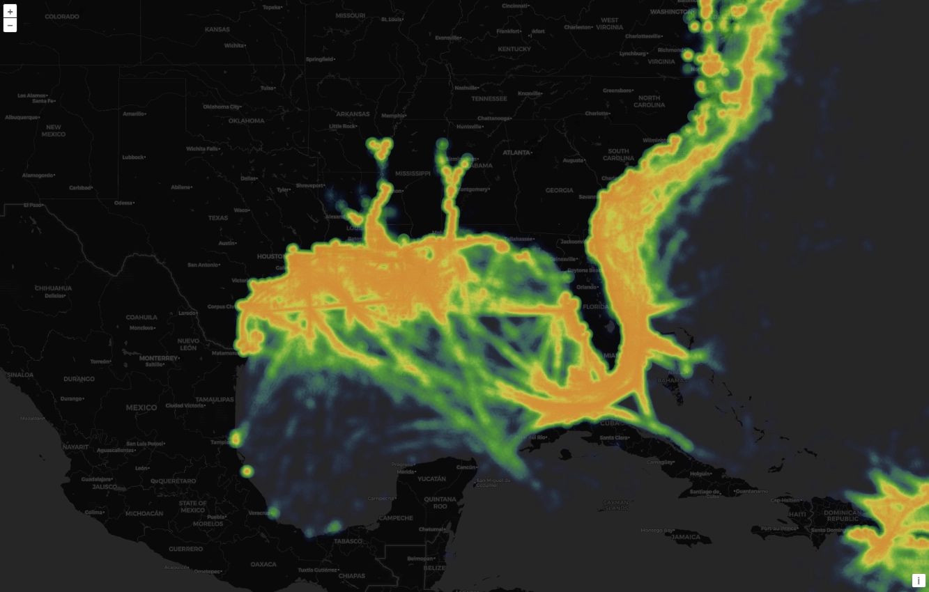
We've got time and that means a time-series database can really help us get cookin'. A great way to visualize the traffic of any vessel is to output a heatmap of traffic via latitude and longitude coordinates. That'll show us via "heat" where ships gravitate.

We'll do so for a year:

SELECT
    latitude,
    longitude
FROM
    vessels
WHERE
    timestamp IN ('2022-01;1M')

This is how it looks in the Gulf of Mexico:

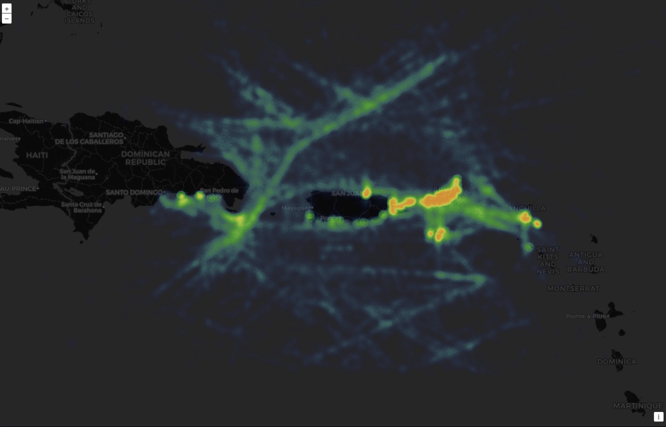
And next is a zoom around the Dominican Republic. It highlights what probably is a main traffic route between the two islands, probably from/to the Panama canal:

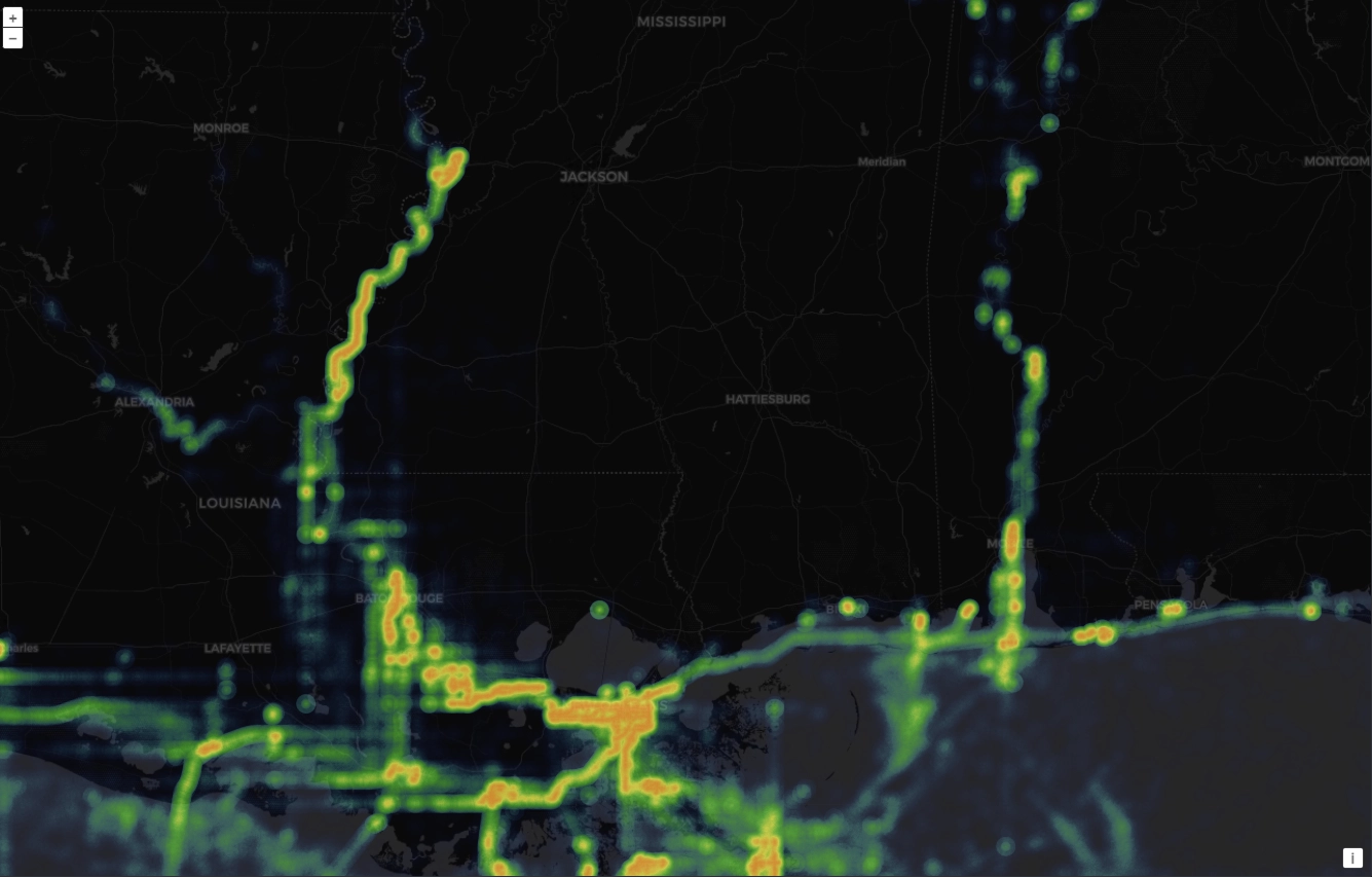
Interestingly, we can also see some fluvial traffic originating from the rivers, particularly into the Mississippi to the port of Vicksburg:

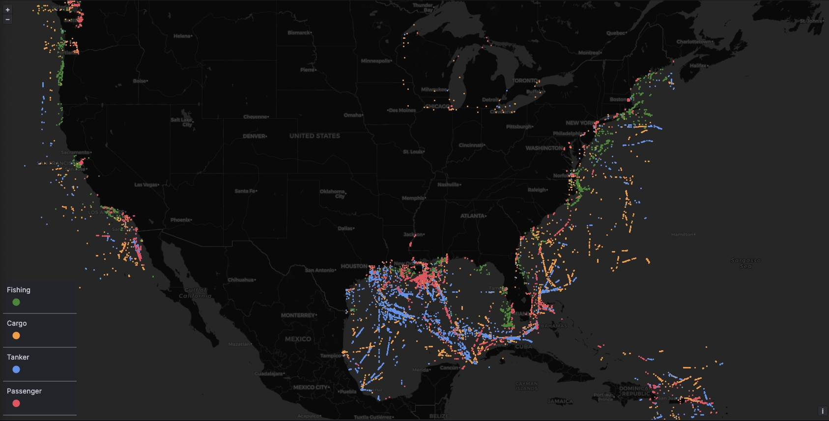
Tracking ships by ship type​

There are many ships out there, sailing the seas. After all, ships serve many different purposes. Some are for military, others commerce and tourism, others performing services for other ships. Luckily, our dataset separates by vessel type. As a result, we can examine the paths for different ship types:

SELECT DISTINCT
    vesselGroup
FROM
    vessels

# Returns...
  vesselGroup
  Passenger
  TugTow
  Cargo
  Other
  Pleasure Craft/Sailing
  Tanker
  Fishing

Knowing the ship types can help us look for specific routes. Where are the hot spots for fishing? What are our premier oil shipping routes? Travel?

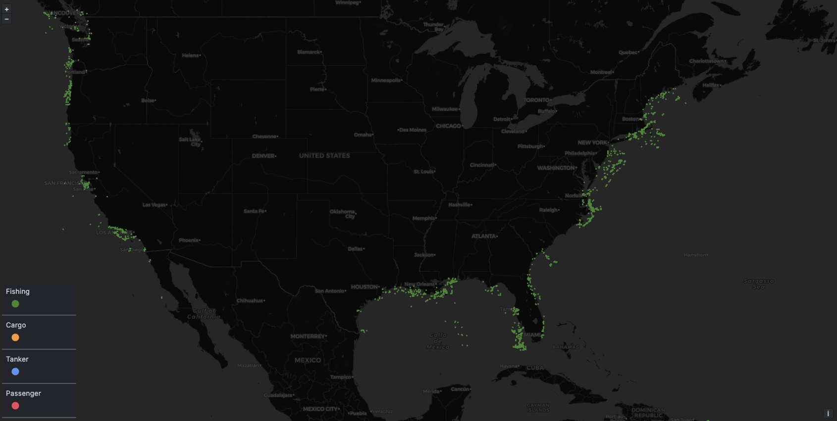
To answer such questions, we can create a few queries to output each vessel type and plot positions on a map. In this case, we are using the limit keyword so as to not overflow Grafana with too much data on a single panel:

SELECT
    latitude,
    longitude
FROM
    vessels
WHERE
    timestamp IN ('2022-01;1d')
AND
    vesselGroup = 'Fishing'
LIMIT
    3000

Now we're talking.

So, about those who fish...

How many of them are coastal?

How many go into deep water?

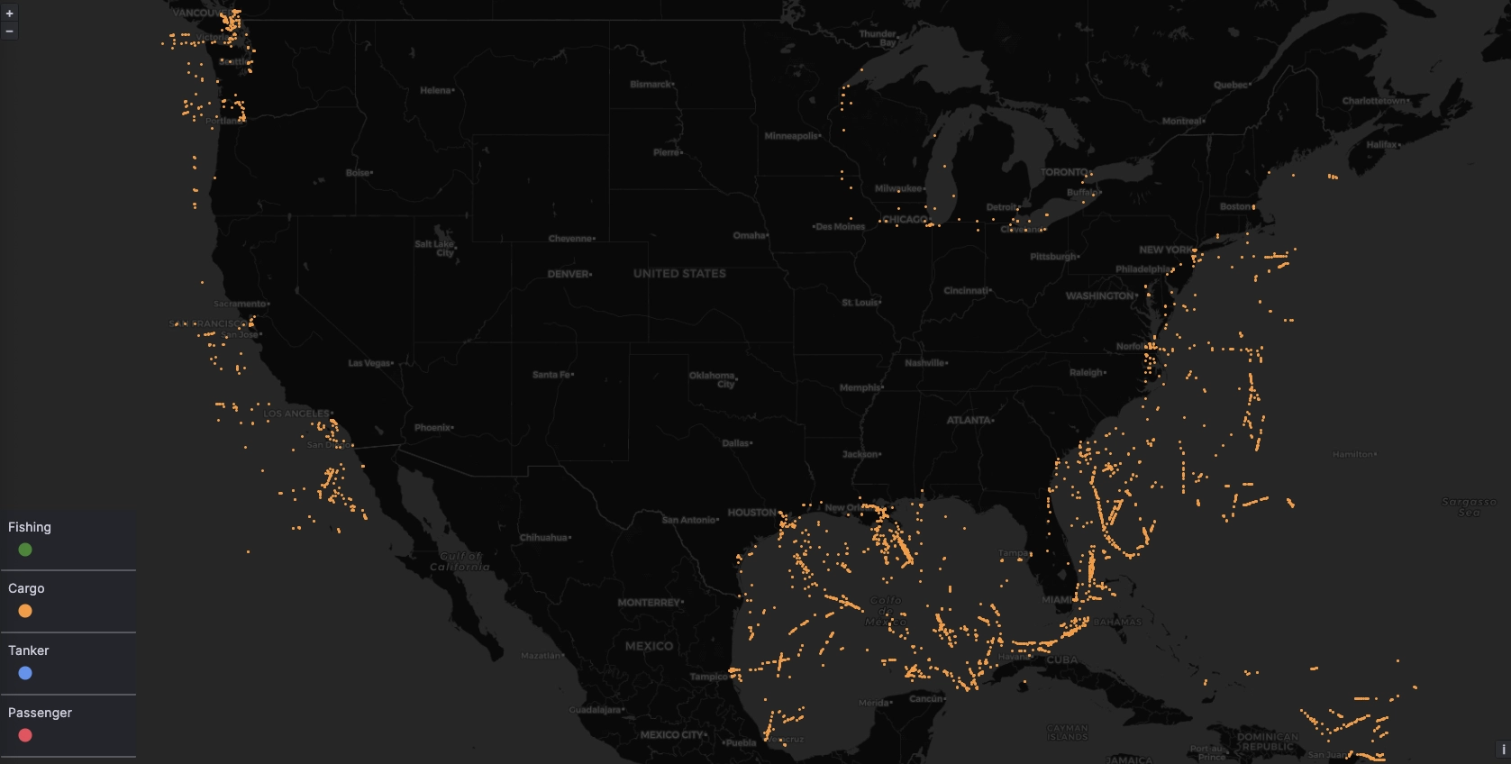
Cargo ships are concentrate on routes to and from the major ports such as Vancouver, LA, Houston, New Orleans and so on. Many are traveling to and from the Gulf of Mexico and are either traveling South to South America or through Panama, or traveling East between Miami and Cuba, likely towards Europe.

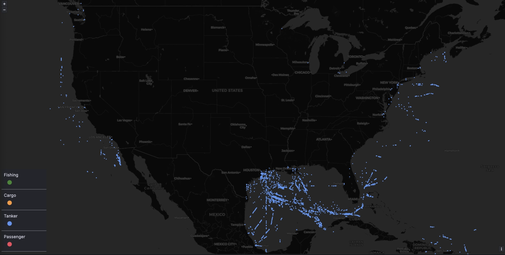
Unsurprisingly, tankers are concentrate heavily around the Gulf of Mexico, particularly around Houston. This clearly shows us that Texas is a major oil hub:

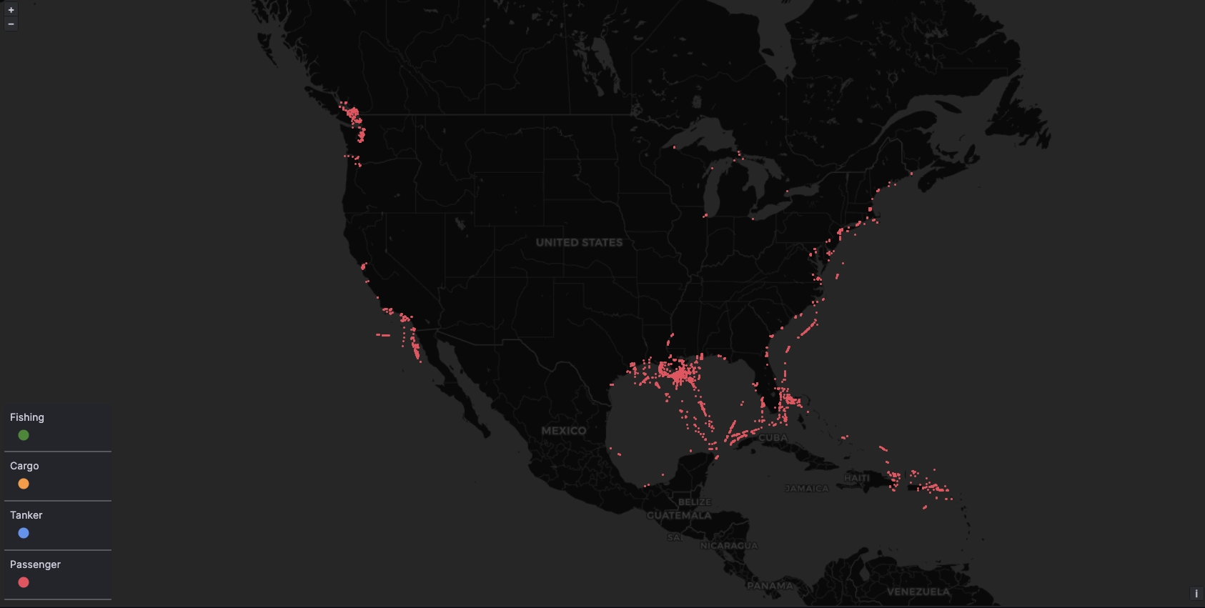
Lastly, passenger transport is centred around hot tourist hubs. There are many routes into the Gulf of Mexico, Cancun, and the Caribbean. Which would be very nice during this cold and rainy time of the UK year...

Following an individual ship​

The MMSI identification number provided by the AIS data is unique to each ship. Through it, we can trace the historical positions of a ship over time.

For example, the ship with MMSI 311050800 traveled from what seems to be the gulf of Yucatan over New Years eve. It then docked in New Orleans and set sail again on January 12th, heading to Miami. After that, it returned to New Orleans towards the end of the month:

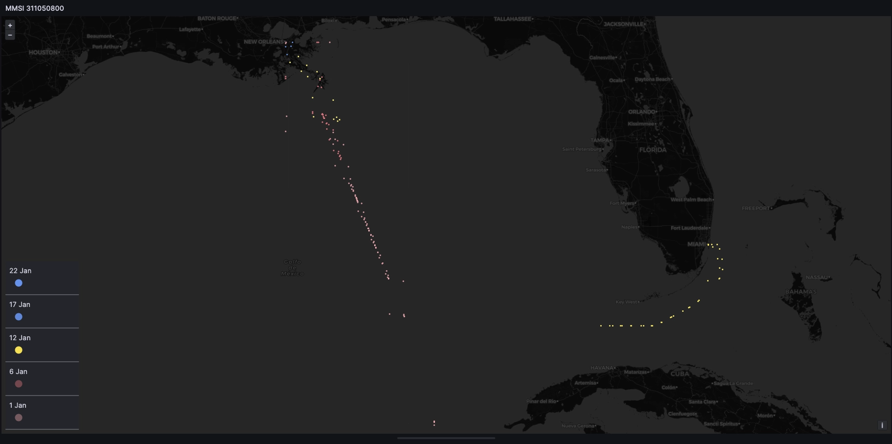
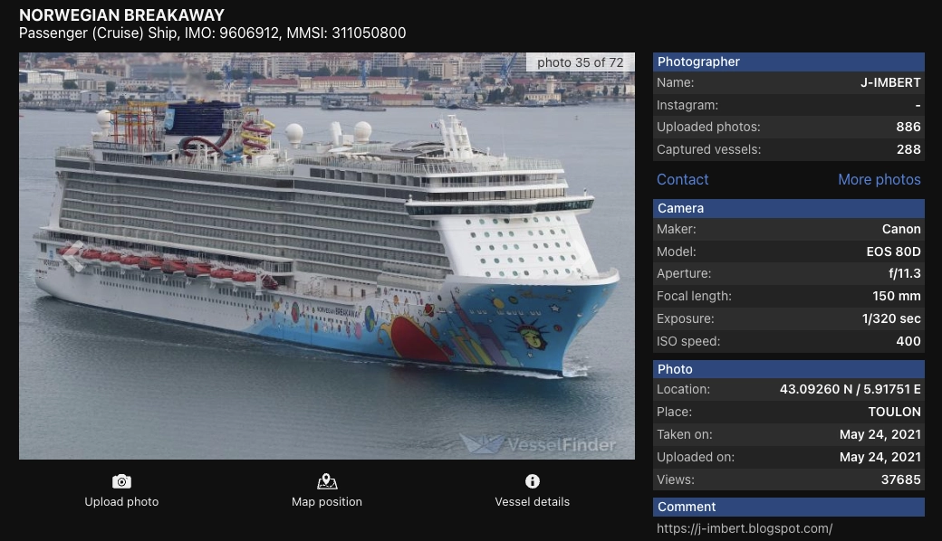
What ship is this, one might wonder? It is the Norwegian Breakaway which seems to currently be cruising around Honduras according to vesselfinder. It even has a water slide. Nice!

Summary​

In this post, we enriched AIS data for nautical vessels then wrote queries to bring the data to life within Grafana. Not all data sets out in the wild are "plug and play". Sometimes it needs grooming. We clarified the set with a few fair assumptions and helper functions.

When analyzing data of this nature, putting it in the context of time opens the opportunity for deep, multi-dimensional analysis. Beneath Grafana we used QuestDB. A specialized database can sail through massive data sets such as this with ease.