
In simple terms, a yield curve is a graph that shows how much money you could earn from an investment over different periods of time. In financial terms, the yield curve is a plot of the yield of fixed-interest securities against the time left to maturity.
The yield curve is major piece of data that underpins most of finance, from mortgage rates to the price of Tesla's stock. In this post, we'll look deeper at what the overall yield curve is and visualise how it changed in the last few years. From there, we'll try to see what it means for the markets overall.
What is the yield, and what does it mean?
The yield of a security is the income derived from holding the security. It is generally expressed in annual terms. For example, consider that an investment costs $97 and that it pays off $100 in 3 months time. The investor purchasing this investment would make $3 on their investment of $97 over 3 months. The yield is therefore $3/$97 = 3.09% for the quarter, or around 12% per annum.
Let's add another layer. Consider if another investment was available paying back $100 in three months, but costing only $95. Then its yield would be 5.26% over the quarter, or around 26% per annum. The reason both investments can exist and have different yields while paying out the same amount at the same time is that they would have different risk profiles. More risk means investors want more reward for taking this risk, and therefore as a result they expect higher yields.
In effect, the yield is a quantity we observe from the prices of different investments. It reflects the amount investors want to earn to buy this investment, as implied by the price at which the investment is trading. Such investment may be a loan and an investor may want more reward for loaning to a "riskier" venture than to an established - and in theory more reliable - business.
The yield curve
In the previous example, we used the yield to compare two investments from two different sources. For example, that could be lending to two different companies or governments or people, and so on, over the same time period. The yield curve is a set of yields for comparable investments in the same entity, but over different time horizons.
For example, you could buy US government debt for $100 face value - effectively lend money to the government - with one year maturity at $95, or with two year maturity at $89. The yield of the first investment is roughly 5.25% while the yield of the second investment is 6.17%.
While the borrower is the same, the yield across the two maturities is different. This difference can have multiple explanations based on the context, but intuitively, one can explain it by the fact that a two year investment locks you up for longer and is therefore riskier.
There is a greater chance that the borrower would default if you lend for a longer term horizon than for a shorter time horizon. For this reason, normal yield curves tend to be upwards slopping; short term yields are smaller than long term yields.
Visualising the yield curve
In this example, we will analyze yield curves from the US treasury website. The dataset contains the rates for each calendar date across a range of tenors, the length of time remaining until a financial contract or agreement expires. It considers one month, 3 months, 5 years and so on.
To import it into QuestDB, download the years in which you are interested from
the treasury website. The files will be in csv format. You can then import
them using the various methods to load a CSV.
As is, the CSV is not directly usable to plot the charts we want in Grafana. We need to change the data a little bit. First, we can rename it for simplicity:
RENAME TABLE 'daily-treasury-rates.csv' TO 'rates'
Second, the table uses one series for each tenor and looks like the following:
| Date | 1 Mo | 2 Mo | ... | 30 Yr |
|---|---|---|---|---|
| 01/26/2024 | 5.54 | 5.45 | ... | 4.38 |
| 01/25/2024 | 5.54 | 5.48 | ... | 4.38 |
| ... | ... | ... | ... | ... |
Ideally, we would not have as many columns. A transformation will make subsequent queries simpler as we would prefer have a table that looks closer to the following:
| Date | Tenor | Value |
|---|---|---|
| 01/26/2024 | 1 Mo | 5.54 |
| 01/26/2024 | 2 Mo | 5.45 |
| 01/26/2024 | ... | ... |
| 01/26/2024 | 30 Yr | 4.38 |
| 01/25/2024 | 1 Mo | 5.54 |
| ... | ... | ... |
To do this, we can create a new table.
We could also complete this with the creation of a designated timestamp. This requires the timestamp field to in ascending order.
Lastly, we can create a new months column of a numeric type as the tenor is
otherwise a string. This is so that we can plot the tenor on an XY scatter chart
in Grafana.
CREATE TABLE yCurve AS (
  SELECT *
  FROM (
    SELECT
      cast(Date as timestamp) timestamp,
      1 months,
      '_1Mo' tenor,
      _1Mo rate
    FROM rates

    UNION

    SELECT
      cast(Date as timestamp) timestamp,
      2 months,
      '_2Mo' tenor,
      _2Mo rate
    FROM rates

    UNION

    SELECT
      cast(Date as timestamp) timestamp,
      3 months,
      '_3Mo' tenor,
      _3Mo rate
    FROM rates

    -- ...

    UNION

    SELECT
      cast(Date as timestamp) timestamp,
      360 months,
      '_30Yr' tenor,
      _30Yr rate
    FROM rates
  )
  ORDER BY timestamp
) timestamp(timestamp);

After these transformations, our `yCurve` table should look like the following:

<Screenshot
  alt="QuestDB interface showing yield query"
  src="/img/blog/2024-01-12/yield-curve-1.webp"
  jumbo={true}
  title="Click to zoom"
/>

We can visualise the yield curve in Grafana as of any date using a query like
the following into a chart which we will call `trends`:

```sql
SELECT months, rate FROM yCurve WHERE Date = '2020-01-02'
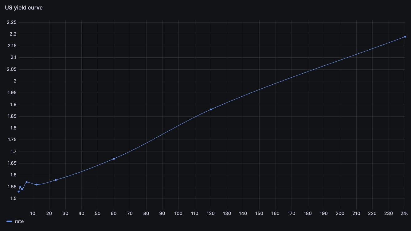
The x axis shows us the months to maturity and the y axis shows the yield/interest rate. This is what a 'normal' curve would look like, roughly. As the investment gets longer, the yield increases. The way to read this is: "As of 02 Jan 2020, investors required a yield of 1.67% on a 5-year investment and a yield of 2.20% on a 20-year investment.
Comparing yield curves
One nice feature of the trends chart template is that it allows us to compare the yield curves as of different dates. For example, we can look at the yield curve at the beginning of Jan and Feb 2020 and compare them in the same chart:
WITH
x AS (SELECT months, rate FROM yCurve WHERE Date = '2020-01-02'),
y AS (SELECT months, rate FROM yCurve WHERE Date = '2020-02-03')
SELECT
  x.months,
  x.rate jan2020,
  y.rate feb2020
FROM x JOIN y ON x.months = y.months
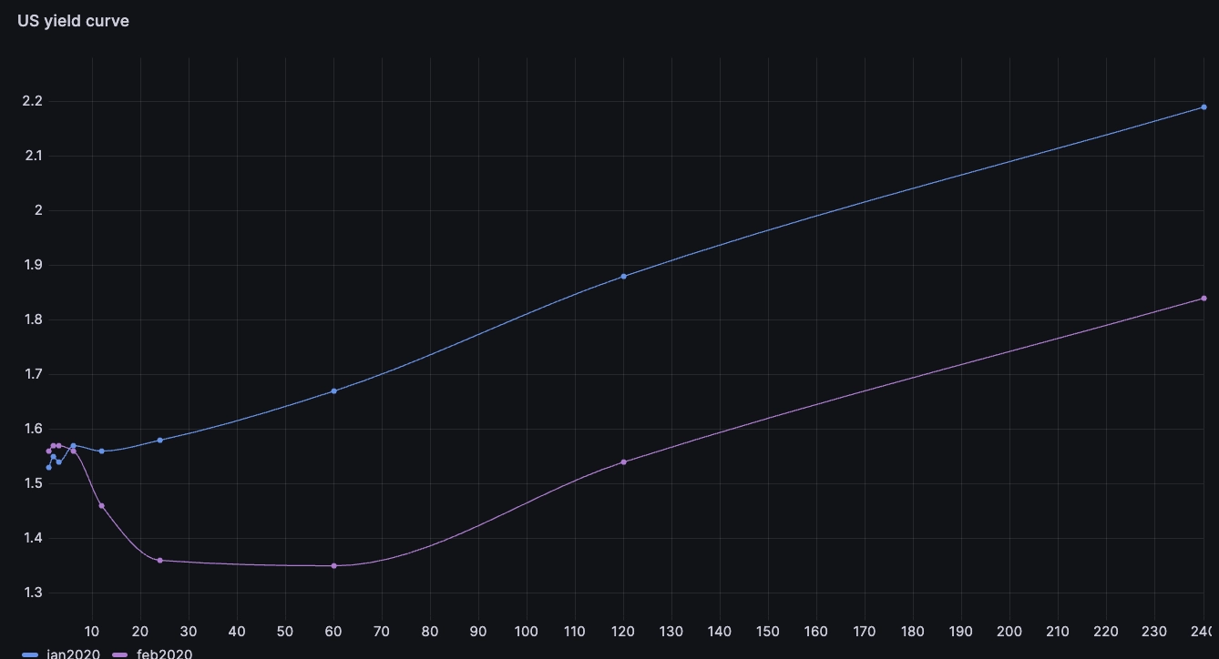
We can see the rates in feb are significantly lower than the rates in Jan over 12 months maturity. This effect is called 'flattening' and can mean investors expect rates to hike and therefore lead to lower economy growth.
Battling COVID
Playing with the same concept, we can look at what happened around March 2020 when the first COVID Lockdowns occurred:
WITH
a AS (SELECT months, rate FROM yCurve WHERE Date = '2020-01-02'),
b AS (SELECT months, rate FROM yCurve WHERE Date = '2020-02-03'),
c AS (SELECT months, rate FROM yCurve WHERE Date = '2020-03-20')
SELECT
  a.months,
  a.rate jan2020,
  b.rate feb2020,
  c.rate mar2020
FROM a
JOIN b ON a.months = b.months
JOIN c ON a.months = c.months
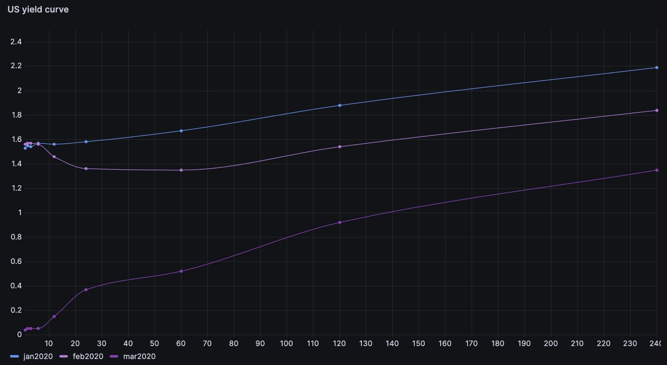
The yield curve is still upwards slopping, but dramatically flattened. The short term yields are near 0. What happened is the US federal reserve cut the interest rates to zero and indicated they would buy government and mortgage bonds. The effect on the yield curve is two-fold:
- The fed rate is the main anchor for all other rates. A Fed rate dropping to zero means all rates drop in parallel.
- The bond buying programme pushes bond prices up. As the bond prices are pushed up, the yields are coming down.
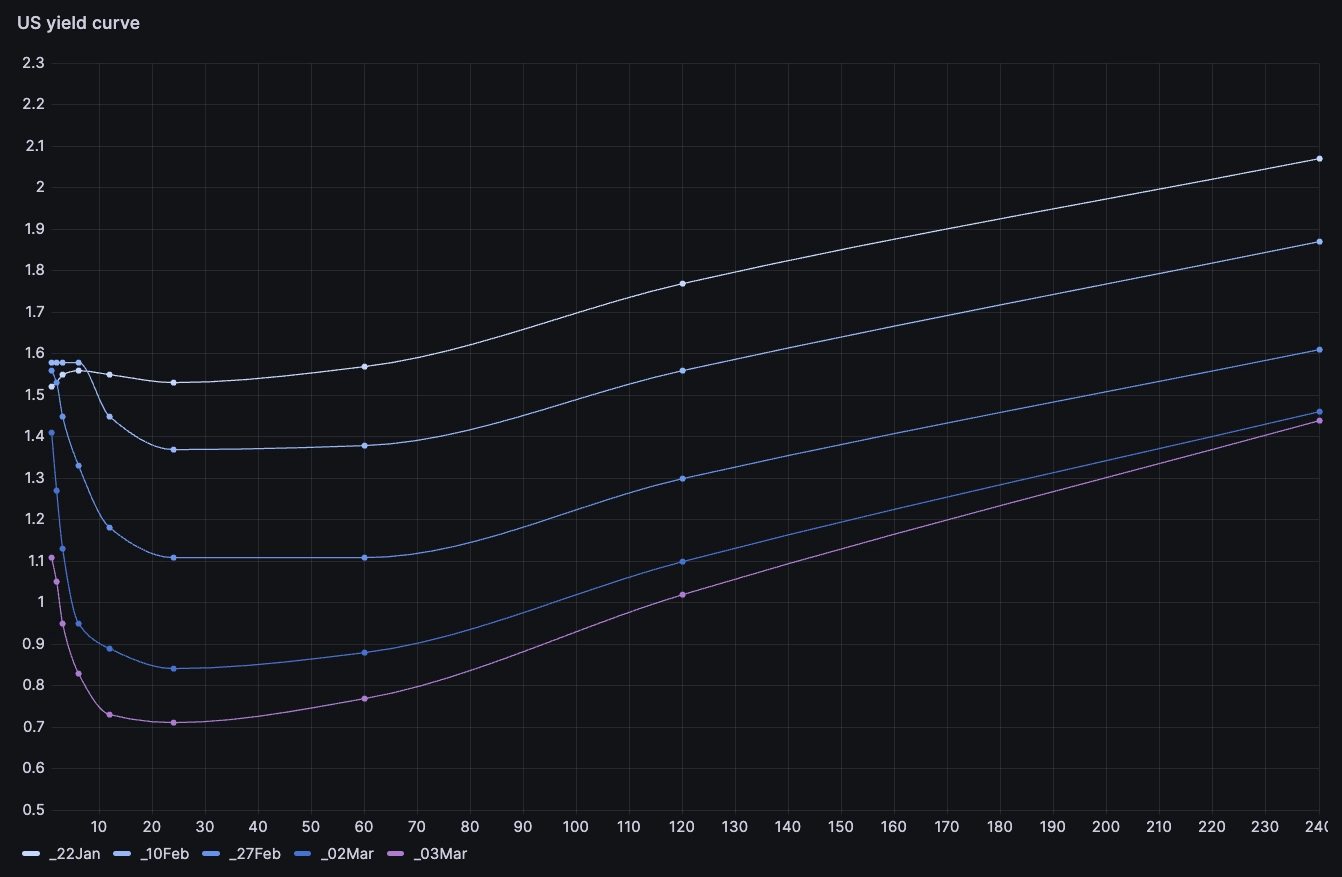
We can see the effect of the announcements - 3 Mar and 15 Mar 2020 - by comparing the curves on the two days surrounding them:
WITH
a AS (SELECT months, rate FROM yCurve WHERE Date = '2020-03-02'),
b AS (SELECT months, rate FROM yCurve WHERE Date = '2020-03-12'),
c AS (SELECT months, rate FROM yCurve WHERE Date = '2020-03-16')
SELECT
  a.months,
  a.rate _2mar2020,
  b.rate _12mar2020,
  c.rate _16mar2020
FROM a
JOIN b ON a.months = b.months
JOIN c ON a.months = c.months
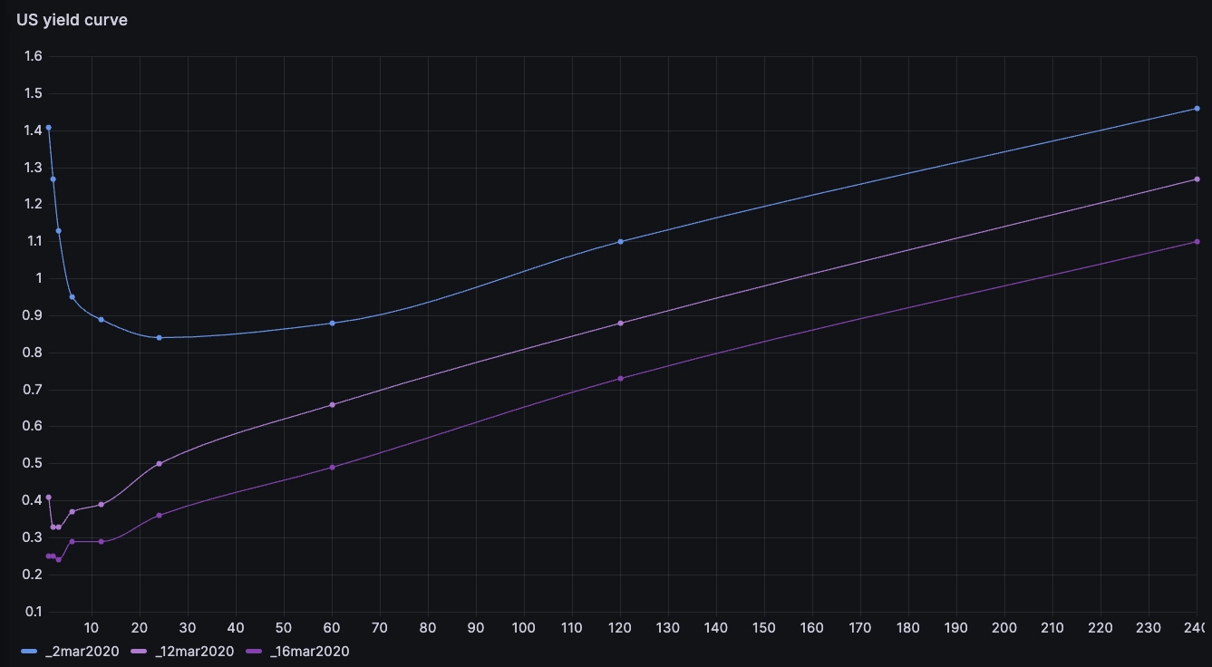
Interestingly, on the day prior to the first rates cut, we can see an 'inverted' curve where short term yields are higher than long term yields. This generally indicates that markets anticipated that the rates would come down in the near future. We can see how this anticipation built up ahead of the announcement:
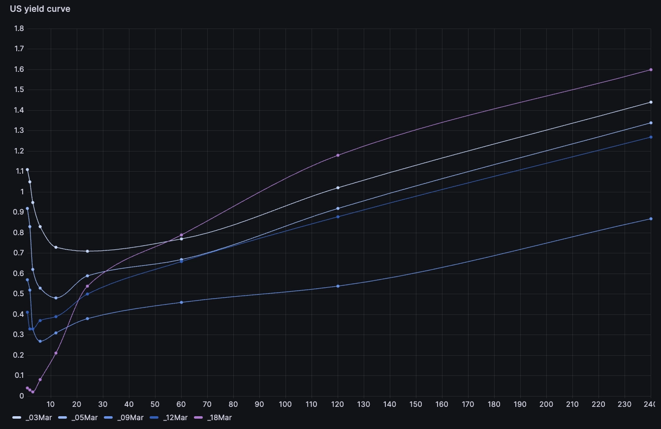
The yield curve went from upward slopping to inverted in the short term and much lower, suggesting an imminent rates cut. In a similar way, we can look at what happened around the 15th March 2020:
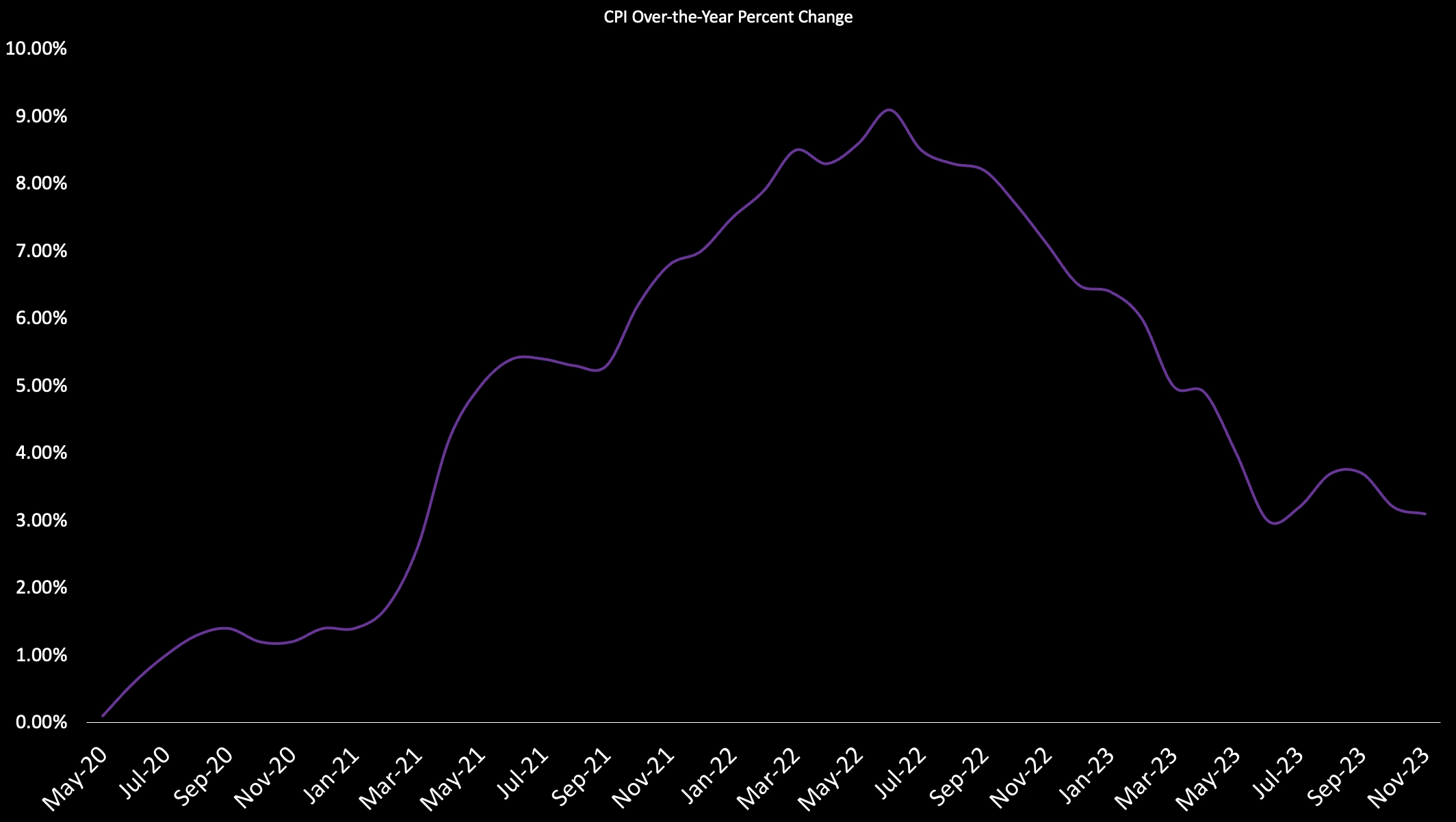
Battling inflation
Starting in 2022, we saw the Fed starting to combat inflation by acting on interest rates. One way to visualise this is to look at the very short term rates over time:
SELECT Date, rate oneMonthYield
FROM yCurve
WHERE tenor = '_1Mo'
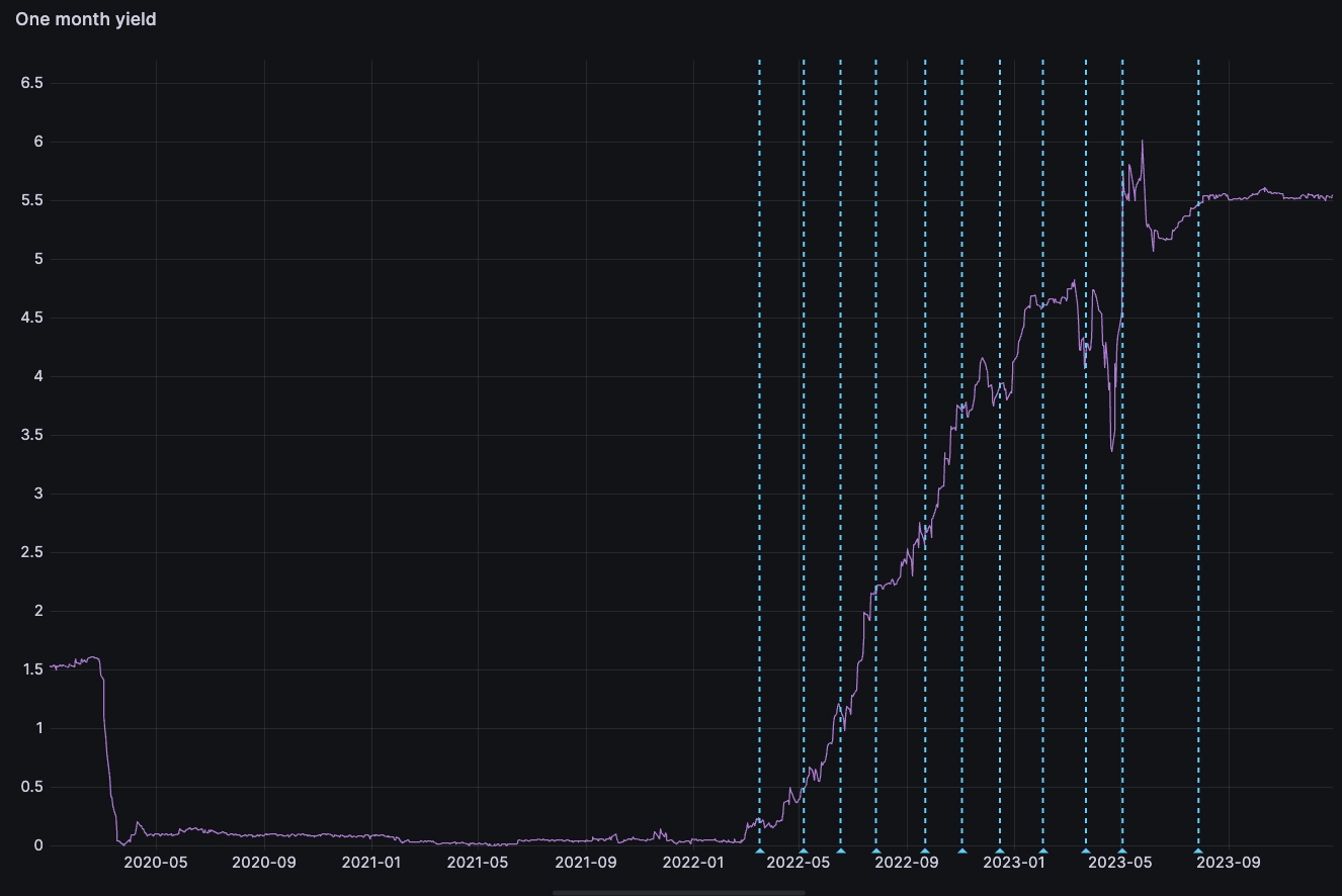
The dashed lines highlight the times where the Fed increased ('hiked') interest rates over 2022 in an attempt to cool down inflation. At the beginning of the period, around March 2020, we can also see when the fed dramatically cut rates and maintained them around 0 during the pandemic.
What to expect now?
By using a similar view, we can overlay the longer term rates and spot inversions:
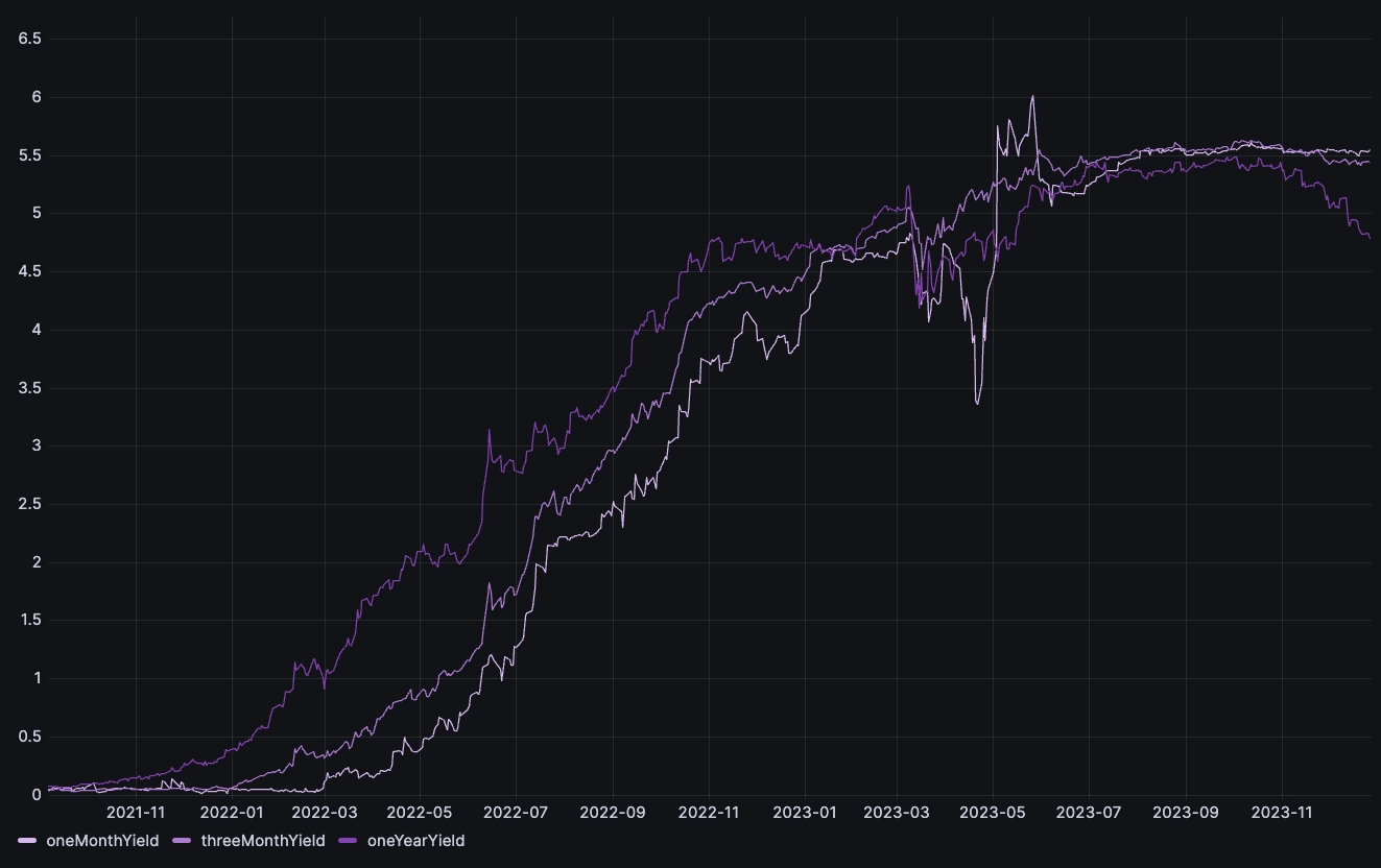
We see that since the summer of 2023, short term yields are higher than the longer term. In other words: the yield curve is inverted. In addition, we can see that inversion seems to be increasing:
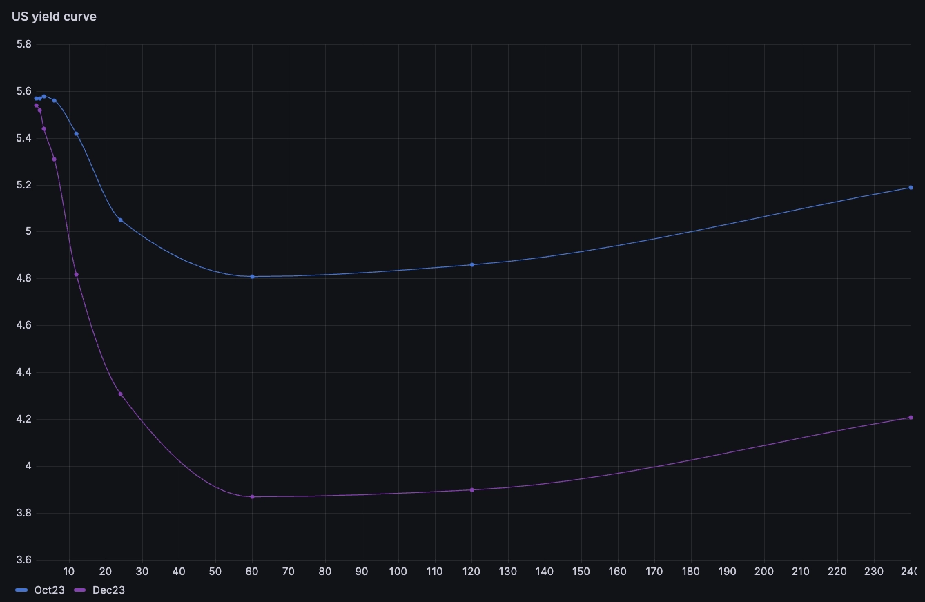
In this instance, we see the longer end of the curve becoming lower while short term interest rates are at the same level or slightly lower. This could indicate a reversal in the current market trend where after almost two years of tightening the monetary policy, the Fed could be expected to start cutting interest rates as hikes seem to have successfully slowed down inflation.
As of Dec 13, the Fed held the rates steady, but indicated three possible cuts over the course of 2023. Above we see how the market anticipated it.
Summary
In this article, we explored the significance of the yield curve in finance, a graph that plots the yields of fixed-interest securities against their remaining maturity. The yield of a security, essentially the income it generates, varies based on the investment's price and inherent risk, reflecting the returns investors expect for different risks.
We then applied time-bound SQL queries to analyze the yield curve in relation to the COVID pandemic. It paints an interesting picture about how markets respond to the rare, real-life events that can influence entire markets.
A time series database like QuestDB when combined with a strong visualization engine like Grafana make a great pair for financial analysis. And isn't the simplicity of SQL easy to understand? Thanks for reading!