NYC taxi meter and options pricing
Every cab I have ever ridden has been complaining about how hard it is to make ends meet as a driver. Using a dataset of over 1.6 billion taxi rides, 700 million FHV rides (Uber, Lyft, etc.), and 10 years of weather and gas prices data, I examine whether the antiquated meter system impacts NYC cabbies' livelihood, rather than competition from the likes of Uber.
A few of months ago, I was putting together data for QuestDB's demo that we shared on ShowHN. It has been a while since I left derivatives trading, and was not expecting to end up writing about options pricing. Much to my surprise, the economics of a taxi meter are very similar to options. This provides an interesting perspective into the fate of taxi drivers.
The economics of the taxi meter
Most rides are priced using the standard meter system. The meter is a machine, which calculates the price of a ride based on inputs such as time, speed, and distance. Additionally, it adds taxes, tolls and surcharges depending on a variety of factors such as the route taken or the time of the day.
Most of the driver's earnings come from the fare, which consists of a
flat fare $2.50 for entering the cab, and a variable fare. The variable fare
is a function of speed, time and distance. It is calculated as follows:
- When the cab drives above 12mph, $2.50 per mile
- Otherwise, $0.50 per minute
This post focuses on the variable fare, i.e the output of the meter excluding
the $2.50 start fee and extras. To be able to compare rides with one another, we
normalize it as an hourly rate of driving a customer around.
Modelling variable earnings for taxi drivers
Let's assume a cab is driving a customer at a constant speed during one hour. At
the end of the hour, the driver can expect to pocket variable earnings of:
- $30 if they drove below 12mph ($0.50 a minute)
- $2.50 x their average speed if they drove above 12mph
Let's plot the hourly earnings in function of speed. This instantly reminds me of an old friend: call options!
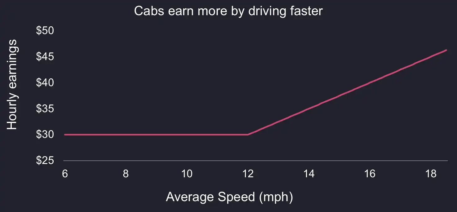
Rewriting the fare formula as follows, we recognize the call option formula
Max(0, S-K).
Hourly Fare = 30 + max(0, Speed - 12)
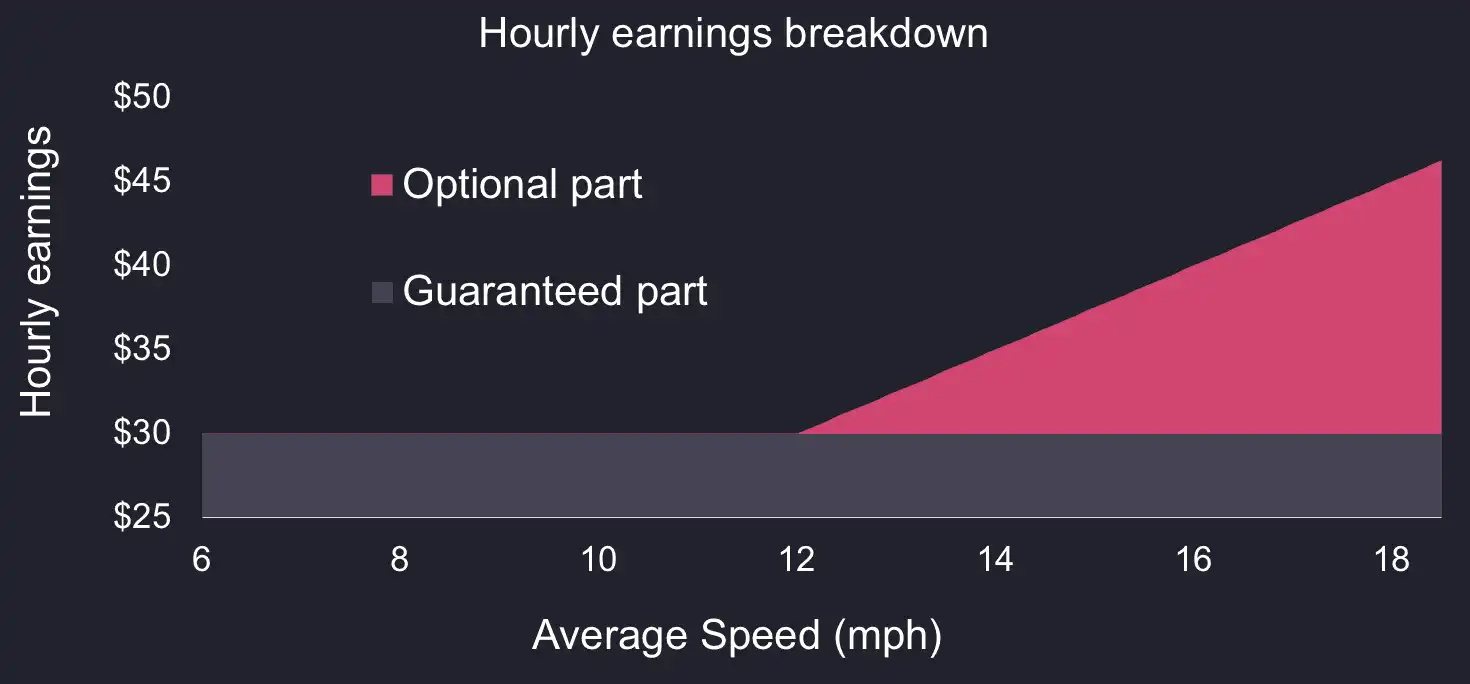
Interestingly, the above notation breaks down the hourly variable fare into two components.
- A
guaranteedcomponent30: whenever driving a customer, a cab will make at least $30 an hour. - An
optionalcomponentmax(0, Speed - 12): driving customers faster earns the driver more.
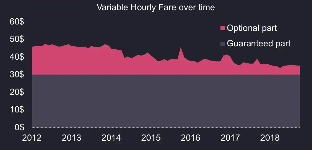
Graphically, the breakdown between guaranteed and optional fare components
look like the below:
There is a reason for this system. It is designed to align the interests of drivers and riders:
- The
guaranteedpart makes discourages riders from making the driver wait and ensures they are paid for their time. - The
optionalpart discourages drivers from purposefully taking customers through traffic.
Let's try to quantify the value of the optional part by using options pricing methods in order to study the incentive for drivers.
A simple approach to options pricing
This post isn’t meant as an essay in financial mathematics (far from it).
However, before we continue, it is useful to understand what makes options
valuable. Buying an option is like paying to play a game with a monetary payout
contingent on some variable.
As an example, think of a dice game. If the die value (our variable) is below 2,
you receive 0. Otherwise, you receive the difference between that value and 2.
In financial markets, the threshold of 2 is known as the strike price and is
denoted K.
You have to pay a fee to play this game. How much are you ready to pay?
To find out, we need to calculate the expected value of a game. This is easy
since we know all possible outcomes and their
respective probabilities of occurrence. We can write these in the table below:
| Dice value | Probability | Payout | Weighed payout |
|---|---|---|---|
| 1 | 16.66% | 0 | 0 |
| 2 | 16.66% | 0 | 0 |
| 3 | 16.66% | 1 | 0.1666 |
| 4 | 16.66% | 2 | 0.3332 |
| 5 | 16.66% | 3 | 0.4998 |
| 6 | 16.66% | 4 | 0.6664 |
By summing all the potential payouts weighed by their probability, we compute the expected value of playing this game: $1.666.
- If we pay less to play the game, we will make money over time.
- If we pay more, we lose in the long run.
This example shows that in its simplest form, the value of an option is equal to the product of the payout profile and the associated probability distribution when the option expires. Let’s visualize this by plotting the values for our game in the following chart:
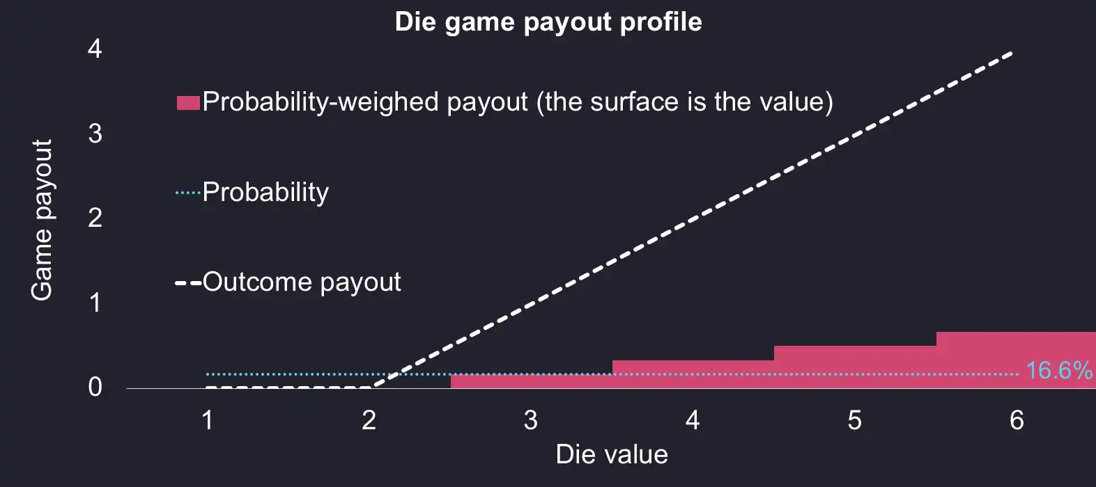
where:
- The white dashed line represents the possible (discrete) payouts for the game.
- The cyan dotted line is the probability for each outcome (dice value) to occur. It is a straight line at 16.66% since each of the 6 values is equiprobable.
- The coloured area is the product of the first two lines. Its total surface is the value of our option.
Of course, this is very simplified. I omit time value, which is the idea that you (almost) always wish you could hold the option for longer. The reason time value exists has to do with the asymmetric payoff profile: there is more to win than to lose by waiting a little longer. Also, in real life, outcomes are rarely equiprobable. For example, stock prices are represented as a log-normal distribution. Nevertheless, this example gives a good introduction to calculate the value of an option.
Now, since we saw that speed is the main driver behind the variable fare, we should attempt to build a representation of speed distribution in order to estimate the option value.
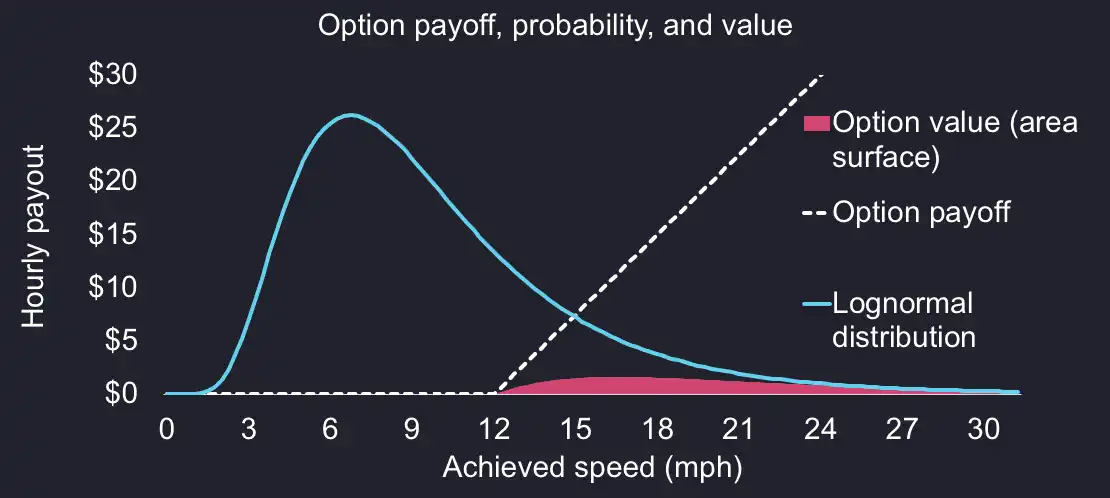
Modelling cabs speed and option value
This can be done using a log-normal distribution, which is analogous to the normal distribution, but cannot be negative. This fits our situation well since cabs can only drive above 0mph.
The log-normal distribution requires two parameters:
- the
mean, i.e a driver's expected average speed for a given hour. - the
standard deviation, a measure of how much the achieved speed is likely to deviate from the mean.
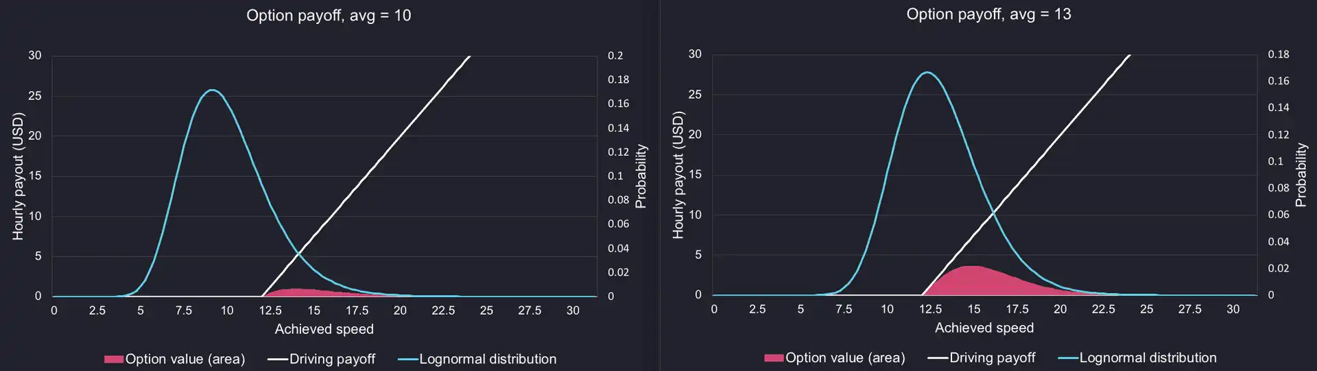
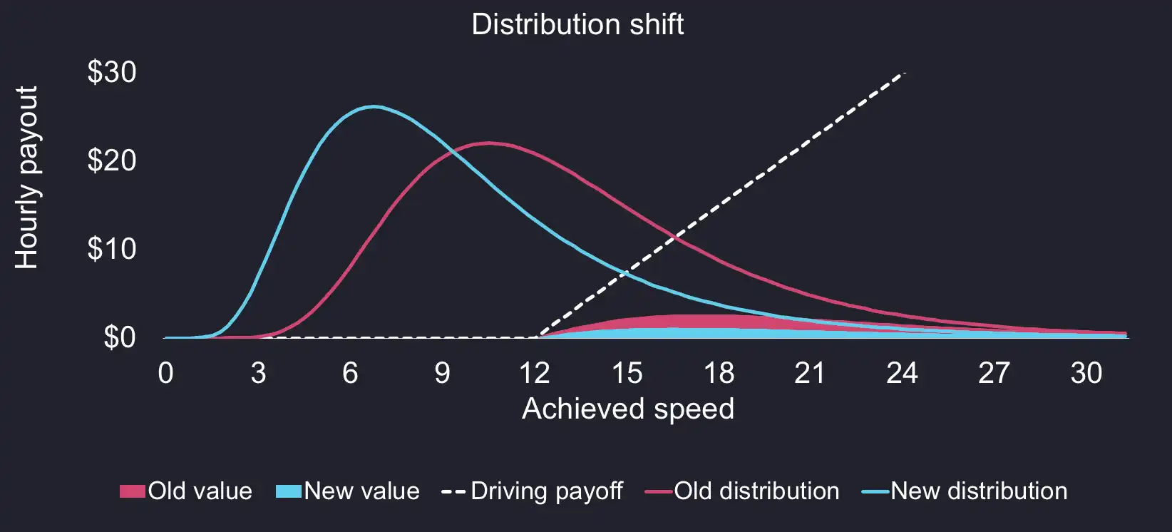
If we overlay the log-normal distribution to the option payoff, we can see the option value below as the product of the two surface areas. As you can see, the log-normal distribution is skewed to the left and the mode (the highest point on the distribution, at around 10 mph) is lower than the mean (13 mph in the above).
We can play with our two parameters to get a grasp on the pricing dynamics. Here is how the average speed changes the distribution and expected option value:
And here is the effect of standard deviation:
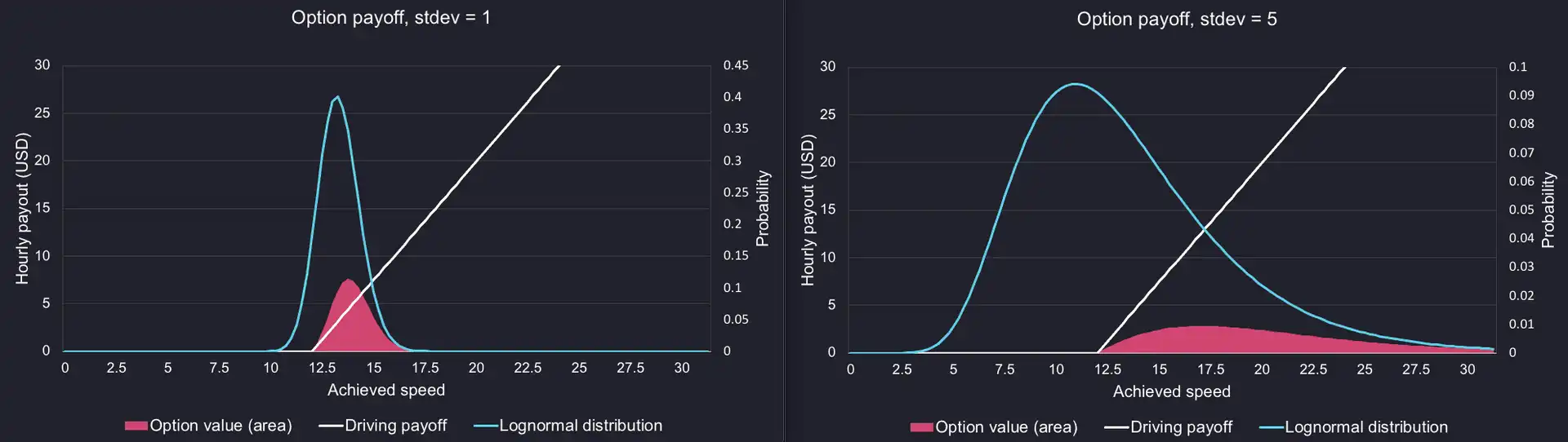
We can see that a higher mean and a higher standard deviation result in higher option value. In short, this means that it is in the drivers' best interests to
- drive faster;
- deviate for the mean, for example by taking risks.
Now, to be clear, I don't mean that they should drive recklessly, but rather that they should attempt "risky" routes, which could either save a lot of time, or otherwise be a disaster.
In traditional finance, the sensitivities to input parameters, which we have introduced above are called the “Greeks”. These are measures of risk named (mostly) after Greek letters. They are used to evaluate and manage the risk of options portfolios. Here are the two greeks respective to the mean and standard deviation:
- The
delta, change of option value relative to change of the mean - The
vega, change of value relative to the change of standard deviation (aka volatility).
These are "first order" greeks, which means they directly affect the option
value. There are more greeks, of higher order, which affect the option value
indirectly. As example, the vanna is a second-order greek which measures how
much the delta (first order greek) of an option changes when volatility changes.
Traffic increase has cost a great amount to taxi drivers
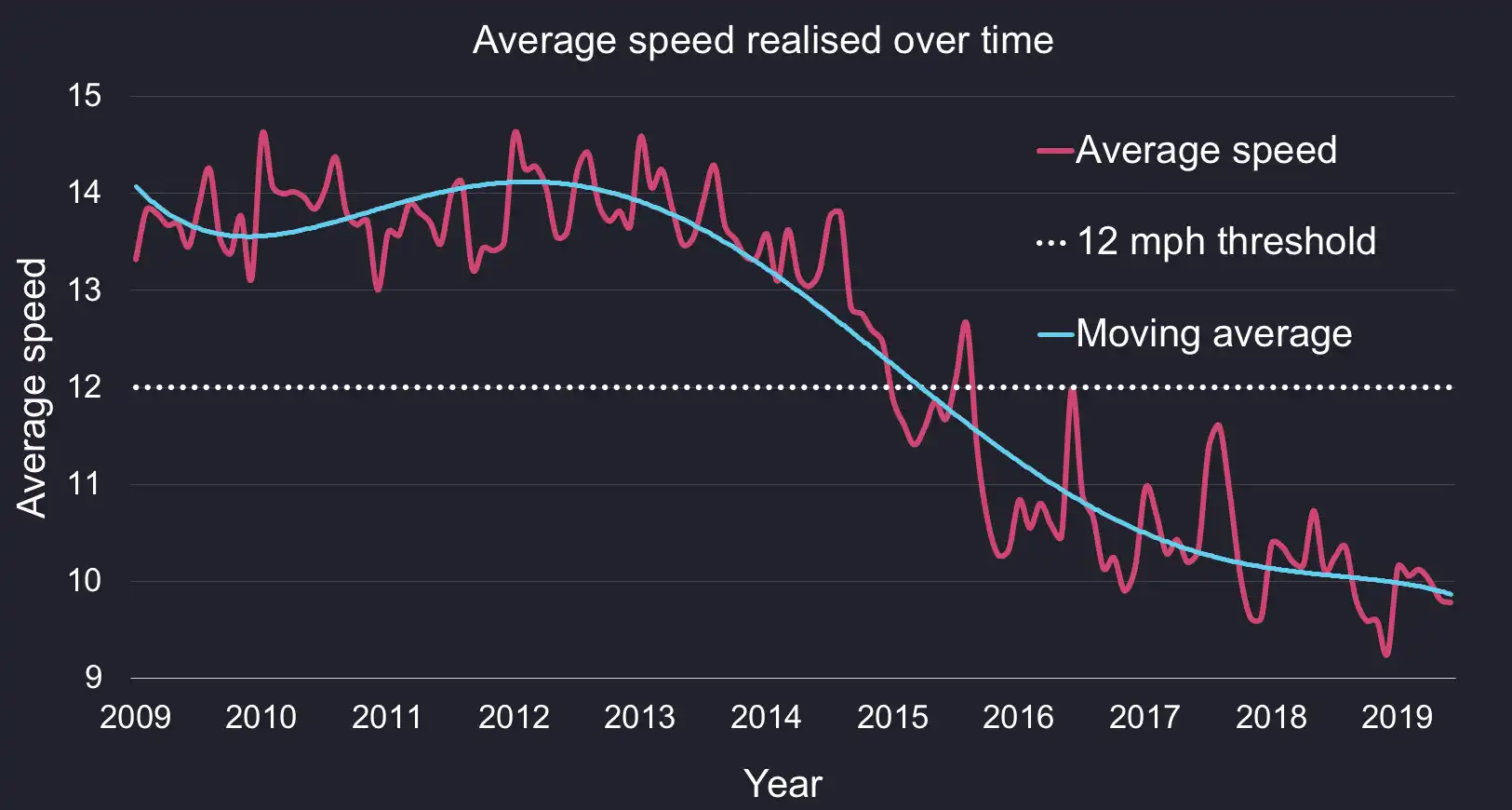
Let’s first look at the average speed over time.
The NYC taxi dataset gives us the distance calculated by the meter, the pickup timestamp, and the drop-off timestamp. Using QuestDB, we can derive the duration of each ride as the difference between the two timestamps and divide the distance by the duration, to calculate the average speed.
With SAMPLE BY, I compute the average results for monthly intervals and plot
it below. Over 10 years, the average speed dropped significantly from 13.3 to
9.7mph (almost 30%!).
This number is a simplification since it assumes constant speed and no idle time. However, it is useful to calculate a lower-bound for earnings as follows.
Min Hourly Variable Fare = Max($30, Avg(speed) * $2.5)
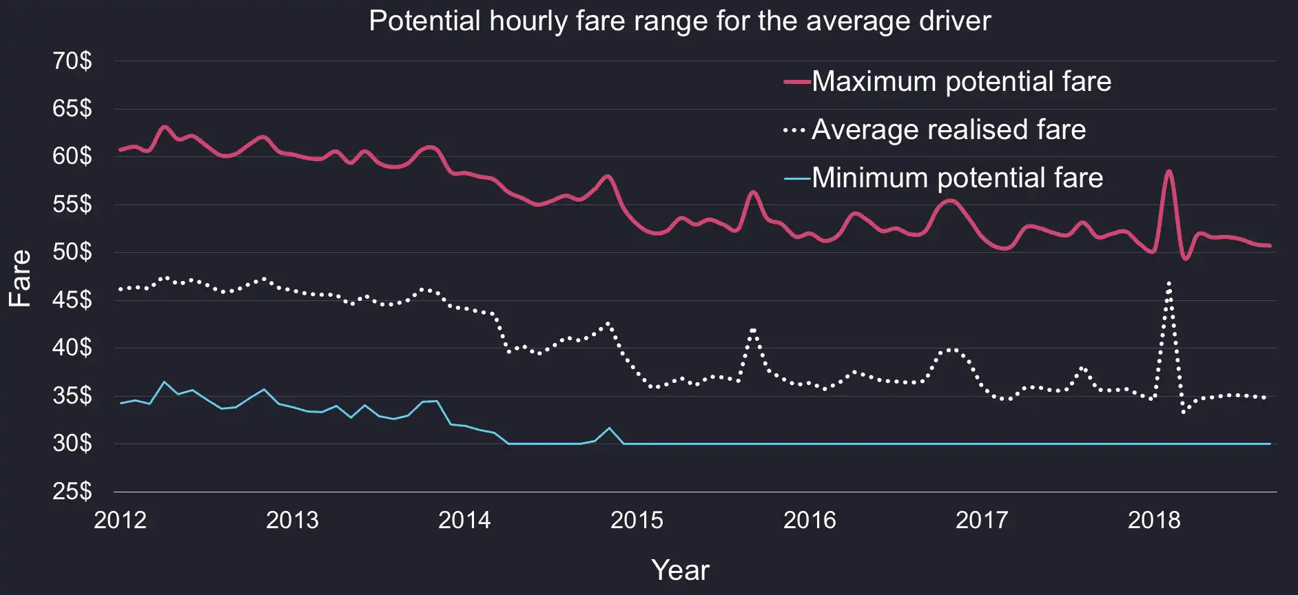
Similarly, we can estimate the upper bound of a driver’s hourly earnings in a theoretical world where drivers are either idle or accelerate instantly from 0 to the speed limit of 25mph. This is how the maximum potential fare could be calculated:
Max potential hourly variable fare = Distance component + Idle component
Distance component = Average ride distance * $2.50 / Average ride duration (hours)
and
Idle component = (25 - Average ride distance)/25mph * 60min * $0.50
Lastly, we can calculate the actual average variable fare over time as follows.
Actual Hourly Variable Fare =avg(fare_amount - $2.50) / avg(duration_hours)
Here is what the three metrics look like over time (note we started the plot in September 2012 since cab prices were increased in August 2012. Interestingly, the average minimum variable fare has dropped over time and is now hitting a floor.
Now that we have the average speed, we can use the standard deviation to model the speed distribution. By feeding the historical mean and standard deviations into a log-normal distribution model, we can compute the following percentiles. For the vast majority of rides, drivers can expect to average below 12mph.
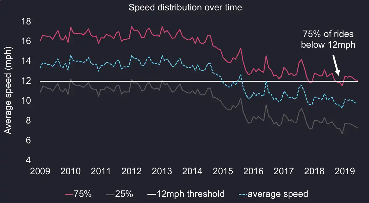
To sum up, the following chart shows how the economics have changed over time. We can see how this damaged the option value for drivers, mostly as a result of the lower trending mean.
We can now use our data to extract the actual option value from the fare as follows.
Option value = Hourly variable fare - Guaranteed component
Option value Actual = Actual Hourly Variable Fare - $30
Slowly but surely, it stopped being a significant part in the driver’s earnings.
I don’t have the data to tell why the average speed is lower, but I would intuitively attribute this to more vehicles on the road as a result of Uber, Lyft, and other FHV, along with urban planning, for example cycle lanes making for less space on the road and more congestion.
Whatever the underlying reasons, the impact is visible, and it is significant. Over the past 10 years, slower traffic has cost up to $10/hour per taxi. To put this in context, this means $29,000/driver each year (8 hours a day, no holidays), or $300 million a year for the entire NYC cab industry! And these are lower bound numbers. In reality, drivers share cabs. If we assume all of the 13,500 cabs are constantly on the road, this adds up to $1.2 billion a year lost for the industry!
Customers are losing too
The pricing system was designed to motivate drivers and riders to play fair. These incentives are almost gone today, which makes the meter system counter-productive.
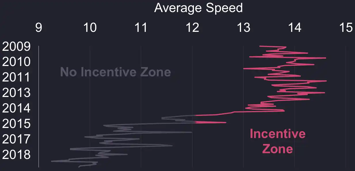
When the average driver could expect to drive at 13mph 10 years ago, their expected speed is now around 9mph, way below the 12mph threshold. The loss of incentive becomes apparent if we look at it over time as follows:
So, are there any reasons left for cabs to drive customers around faster?
The start fee of $2.50 provides another incentive. But it's efficacy depends on the waiting time between two rides. If the expected wait between customers is 5 minutes or less, then drivers remain incentivized. Otherwise, it is economically more efficient to drive slowly and make the most of the current customer. A slow-earning loaded cab makes more money than an empty one.
I don’t have data to estimate the waiting time for drivers between two rides. But in a world with increased supply and competition (Uber, Lyft etc.), I think it is safe to assume that the wait time for drivers has increased. So while I cannot tell for sure if the start fee has lost all of its incentive, it seems fair to say that it lost a good part of it.
If drivers are uncertain about their likelihood of finding the next ride, and if the optional fare component has become an insignificant fraction of their earnings, then it makes more sense to drive slow, and to hold on to the current customer for as long as possible. In the end, $30 per hour is better than 0.
Your turn to explore the data
We made this dataset and the database available online and you can query it directly from your browser via QuestDB demo.
Feel free to explore it, come up with more analysis, and let me know your findings.
I am particularly interested in expanding these results based on weather data. I let readers give it a try using the hourly data available on the QuestDB demo server. In his analysis, Todd W Schneider concluded that the rain had no significant impact on the number of rides. But what about the fare value? Doesn't it feel like when it's raining, traffic gets slower? It would be interesting to study how the weather affects a driver's speed, and in turn earnings. This is only one of the so many fascinating questions left to explore with this dataset.
Anyway, I hope you found this interesting. If you like this post, please consider leaving a star on our GitHub. And, if you find anything interesting while playing with the data, email me and we'll write about it!