Demo geospatial and timeseries queries on 250k unique devices
The last significant features we shipped dealt with out-of-order data ingestion, and we focused our efforts on hitting the highest write-throughput that we could achieve for that release. Our latest feature highlight adds space as a new dimension that our database can manage and allows users to work with data sets that have spatial and time components.
We shipped an initial implementation with software release version 6.0.5, and we've updated our demo instance so anyone can test these features out. To help with running queries on this sort of data, we've included an example data set which simulates 250,000 moving objects, and we've provided examples in the SQL editor to demo common types of queries.
This blog post is mainly for people who work with geospatial data struggling with performance, are looking for new tooling, or need to track changes in geodata over time. This post should also be interesting for those who want to read about how we added geospatial support to our time series database from a technical perspective.
What are geohashes?
Geohashes work by dividing the Earth into 32 separate grids, and each grid is assigned an alphanumeric character. We can increase the precision by sub-dividing each grid into 32 again and adding a new alphanumeric character. The result is a base32 alphanumeric string that we call a geohash, with greater precision obtained with longer-length strings.
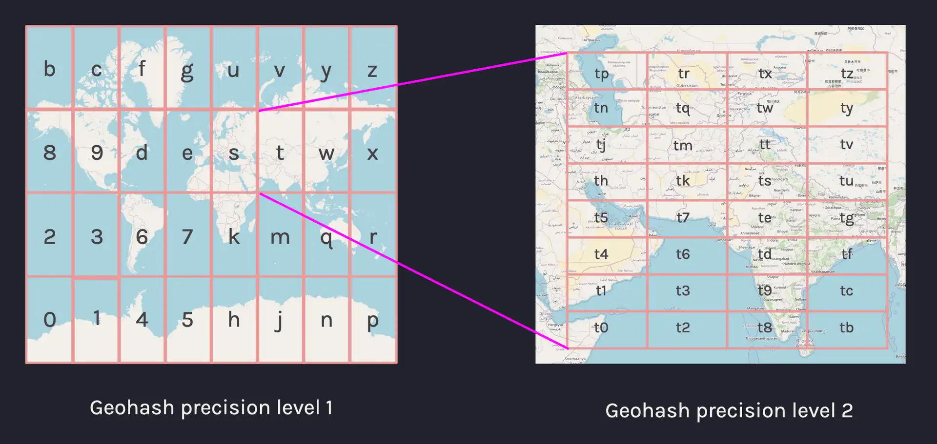
To support geospatial data, we added a new geohash type which would allow
special handling of geohashes. We'll take a look at the syntax we introduced in
the language additions section below, but
first, let's get an idea of what a geohash represents in terms of geographic
area, we can take a few examples and compare the resulting grid size:
| Type | Example | Area (precision) |
|---|---|---|
geohash(1c) | u | 5,000km × 5,000km |
geohash(3c) | u33 | 156km × 156km |
geohash(6c) | u33d8b | 1.22km × 0.61km |
geohash(12c) | u33d8b121234 | 37.2mm × 18.6mm |
Mapping geohashes
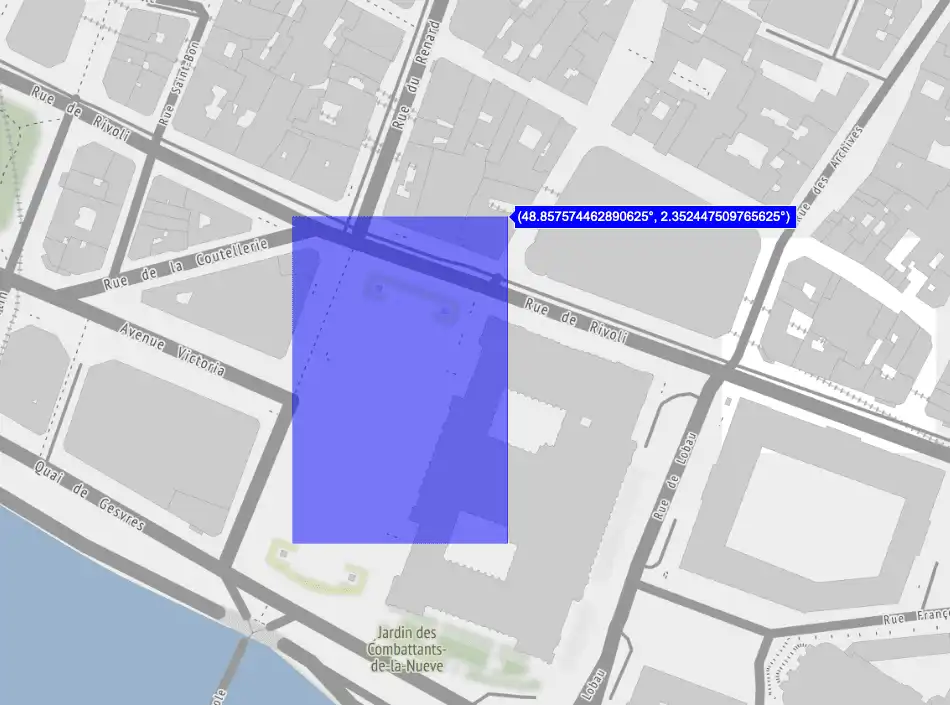
To place geohashes on a map, we need to know the bounding coordinates of the corners of each grid. There's a very helpful script by Chris Veness that allows users to input latitude and longitude coordinates and maps the equivalent geohash. In this case, the precision of the returned geohash is based on the decimal places of the lat/long coordinates.
The inverse calculation from geohash to latitude and longitude follows a similar logic but instead requires creating a bounding box comprising four corners of the grid. To calculate the geohash bounding box and place it on a map, we can use a function similar to this example:
# calculates the lat long bounds of a geohashdef bounds(geohash):base32 = '0123456789bcdefghjkmnpqrstuvwxyz'evenBit = TruelatMin = -90latMax = 90lonMin = -180lonMax = 180for char in geohash:idx = base32.index(char)for n in range(4, -1, -1):bitN = idx >> n & 1if evenBit:# longitudelonMid = (lonMin+lonMax) / 2if (bitN == 1):lonMin = lonMidelse:lonMax = lonMidelse:# latitudelatMid = (latMin+latMax) / 2if (bitN == 1):latMin = latMidelse:latMax = latMidevenBit = not evenBitbounds = {'sw': (latMin, lonMin), 'ne': (latMax, lonMax)}return boundsprint(bounds('u09tvw0r2'))# {'sw': (48.85744571685791, 2.3514175415039062), 'ne': (48.85748863220215, 2.3514604568481445)}
Once we have the coordinates in latitude and longitude, we can use standard mapping tools to visualize geohashes by creating bounding boxes like the following example, which uses plotly via Python:
QuestDB geohash syntax and storage
The syntax we chose for column definitions follows the format
geohash(<precision>) where precision can be between one and twelve characters
or directly binary values. Precision is specified as n{units} where units
may be either c for char or b for bits (c being shorthand for 5 x b).
For example, the geohash u33d8b is represented by six characters, so we can
store this in a geohash(6c) column.
We decided against using strings to represent geohash values as this is
inefficient for both storage and value comparison, so we chose to add geohash
literals. The literal syntax that we use has the format of a single # hash
prefixing the geohash value for chars and two ## hashes for binary:
-- Create two geohash columns with different precisionCREATE TABLE geo_data (g5c geohash(5c), g29b geohash(29b));-- Inserting geohash literalsINSERT INTO geo_data VALUES(#u33d8, ##10101111100101111111101101101)-- Querying by geohashSELECT * FROM geo_data WHERE g5c = #u33d8;
In terms of storage for geohash values internally, we use four different categories based on how much storage each geohash would require. We break geohashes down into the following types internally:
- Up to 7-bit geohashes are stored as 1
byte - 8-bit to 15-bit geohashes are stored in 2
bytes - 16-bit to 31-bit geohashes are stored in 4
bytes - 32-bit to 60-bit geohashes are stored in 8
bytes
There may be cases where you need the control over storage provided by binary
values but would prefer to work with character-formatted geohashes. We can do
this by including a suffix in the format /{bits} where bits is the number of
bits from 1-60. This way, you can choose specific binary column precision for
storage, but the values passed around use char notation with lower precision:
-- insert a 5-bit geohash into a 4 bit columnINSERT INTO my_geo_data VALUES(#a/4)-- insert a 20-bit geohash into an 18 bit columnINSERT INTO my_geo_data VALUES(#u33d/18)
Optimizing for common usage patterns
Adding space as a dimension was one side of the problem, but we considered that many use cases would track moving objects, and common usage patterns would likely require more than optimized storage and ingestion only. Tracking moving objects, for instance, is a different problem than stationary entities with a fixed location (like a lookup table). We wanted to enable users to have performant query execution on the change of location of an entity over time. Optimizing these kinds of queries has two obvious solutions:
- perform a geohash lookup first, then search these results by time, or
- search the data by time range, then perform a geohash search within the results
We benchmarked these scenarios and chose a time-based search first, followed by geohash lookup for performance reasons, as we avoid scanning all non-indexed rows first. Because timestamp columns are already indexed, we leverage high-performance time-based search and filter the resulting (smaller) data sets. The most significant performance penalty that we incur is lifting data from the disk in the first place, so we try to avoid this.
Functions and operators
We focused on internal optimizations for the first() and last() functions
used in aggregate queries to make them execute faster. The optimization is
currently restricted to SAMPLE BY queries, and the functions need to be called
on symbol types with an index. The result is that there is a faster execution
time when you would like to retrieve the first or last-known value for a given
object (symbol) within an aggregate bucket.
To illustrate why this is useful, one example on our demo instance uses
SAMPLE BY 15m to split the results into 15-minute aggregate buckets. When we
use the last(lat) function here, we avoid lifting all data from the disk for
the lat column, but instead read the row ID based on the timestamp index and
instead pick the last value within our aggregate bucket:
SELECT time, last(lat) lat, last(lon) lon, geo6 FROM posWHERE id = 'YWPCEGICTJSGGBRIJCQVLJ'SAMPLE BY 15m;
In order to take a snapshot of moving objects within a certain area, we
introduced a within operator which evaluates if a comma-separated list of
geohashes is equal to or within another geohash. This operator works on
LATEST BY queries on indexed columns, the device_id column in this snippet,
for example:
SELECT * FROM pos LATEST BY idWHERE geo6 within(#ezz, #u33d8);
The implementation of within was designed to be used with additional
time-based filtering, so that we can efficiently sample data sets in terms of
time and space. The query performance of slicing time and space in this way
should be fast enough to power real-time mapping tools which make use of UI
sliders to jog through slices of time:
SELECT * FROM pos LATEST BY idWHERE geo6 within(#wtq)AND time < '2021-09-19T00:00:00.000000Z';
We wanted high-performance prefix-based searches that can execute across
hundreds of thousands of unique values for this operator. To perform this in a
non-naive way, have a 'map-reduce' approach which splits keys into groups and
performs operations upon such groups in parallel. For within, a task
processing queue slices a range of geohashes, and our worker pool performs
prefix matching:
template<typename T>void filter_with_prefix_generic_vanilla(const T *hashes,int64_t *rows,int64_t rows_count,const int64_t *prefixes,int64_t prefixes_count,int64_t *out_filtered_count) {int64_t i = 0; // input indexint64_t o = 0; // output indexfor (; i < rows_count; ++i) {const T current_hash = hashes[to_local_row_id(rows[i] - 1)];bool hit = false;for (size_t j = 0, sz = prefixes_count/2; j < sz; ++j) {const T hash = static_cast<T>(prefixes[2*j]);const T mask = static_cast<T>(prefixes[2*j+1]);hit |= (current_hash & mask) == hash;}if (hit) {rows[o++] = rows[i];}}*out_filtered_count = o;
We use SIMD across most of our subsystems and use this method for any bulk data processing. The prefix matching illustrated above has vectorized equivalent so that we can perform this search operation massively in parallel:
template<typename T, typename TVec, typename TVecB>void filter_with_prefix_generic(const T *hashes,int64_t *rows,int64_t rows_count,const int64_t *prefixes,int64_t prefixes_count,int64_t *out_filtered_count) {int64_t i = 0; // input indexint64_t o = 0; // output indexconstexpr int step = TVec::size();const int64_t limit = rows_count - step + 1;for (; i < limit; i += step) {MM_PREFETCH_T0(rows + i + 64);TVec current_hashes_vec;for (int j = 0; j < TVec::size(); ++j) {current_hashes_vec.insert(j, hashes[to_local_row_id(rows[i + j] - 1)]);}TVecB hit_mask(false);for (size_t j = 0, size = prefixes_count / 2; j < size; ++j) {const T hash = static_cast<T>(prefixes[2 * j]); // narrow cast for int/short/byte casesconst T mask = static_cast<T>(prefixes[2 * j + 1]);TVec target_hash(hash); // broadcast hashTVec target_mask(mask); // broadcast maskhit_mask |= (current_hashes_vec & target_mask) == target_hash;}uint64_t bits = to_bits(hit_mask);if (bits != 0) {while(bits) {auto idx = bit_scan_forward(bits);rows[o++] = rows[i + idx];bits &= ~(1ull << idx);}}}// for loop same as previous example...*out_filtered_count = o;}
One of the benefits of SIMD-based data processing is that we do not have to rely on external indexes. This follows our original ethos of not introducing additional data structures until absolutely necessary.
What we learned
As we began working with geospatial data sets, we found that there tends to be a lot of data noise in specific scenarios. Specifically, we saw noisy data when objects send location updates but are not moving for a particular time. Our initial implementation does not solve this completely, but we are looking at ways to add mechanisms that discard similar entries within certain bounds to eliminate duplication of records.
When adding our test data set with 250k objects, we estimated the number of unique symbols that QuestDB could easily handle was 100k or less before encountering performance issues. The example data set we are currently using shows that we can store and query up to 250k unique symbol values or more.
Adding support for geospatial data was a great challenge for us, and we think we found novel approaches for the storage model and optimizations for common usage patterns that yielded surprisingly good performance results. We're happy to share our findings, and we're eagerly awaiting feedback on these features, which you can try directly on our live demo or via our latest releases.
If you have have feedback or questions about this article, feel free ask in our Community Forum) or browse the project on GitHub where we welcome contributions of all kinds.