VWAP, or Volume Weighted Average Price, is a cumulative benchmark used to track the price of financial instruments. It represents the average price at which a security has traded throughout the day, adjusted for volume. It can help analysts assess the quality of individual trades or look at the overall trend of the market. VWAP is widely considered as one of the most important benchmarks.
In this post, we will use QuestDB and Grafana to understand how the VWAP algorithmic trading strategy works, and how to calibrate it with the help of volume profiles. The volume profile of an instrument is created by analyzing historical data, and it shows how the overall traded volume is distributed over the trading day.
What is the VWAP trading strategy?
When executing large orders, it is often beneficial to slice the order into smaller chunks over the trading day to avoid adverse price impacts due to lack of liquidity. This is usually carried out by a slicing algorithm, such as the VWAP trading strategy, which aims to match the average execution price of the orders with the VWAP benchmark.
The Cumulative Nature of VWAP
VWAP is cumulative, meaning it aggregates data from the beginning of the trading day up to the current point, providing a rolling benchmark.
The formula for VWAP is:
Calculating VWAP with QuestDB
All the examples below point to the QuestDB Live Demo, with real time ingestion of crypto trades. Give it a go!
The following query calculates the VWAP from individual trades in QuestDB:
SELECT timestamp, cumulative_value/cumulative_volume AS vwap
FROM (
    SELECT timestamp,
           SUM(traded_value)
                OVER (ORDER BY timestamp) AS cumulative_value,
           SUM(volume)
                OVER (ORDER BY timestamp) AS cumulative_volume
    FROM (
        SELECT timestamp, SUM(amount) AS volume,
            SUM(price * amount) AS traded_value
        FROM trades
        WHERE timestamp IN yesterday()
          AND symbol = 'ETH-USD'
        SAMPLE BY 10m
    )
) ORDER BY timestamp;
If we only have aggregated trades data, i.e. candlesticks, we can calculate the typical price for the interval and use that together with the volume. The typical price is calculated as the average of the high, low and closing prices of the instrument during each aggregation interval.
The example below gives an idea how this can be calculated using 10-minute intervals:
SELECT timestamp, first, low, high, last,
    cumulative_value/cumulative_volume AS vwap
FROM (
    SELECT timestamp, first, low, high, last,
           SUM(((low + high + last) / 3) * volume)
                OVER (ORDER BY timestamp) AS cumulative_value,
           SUM(volume)
                OVER (ORDER BY timestamp) AS cumulative_volume
    FROM (
        SELECT timestamp, SUM(amount) AS volume,
            FIRST(price) AS first, MIN(price) AS low,
            MAX(price) AS high, LAST(price) AS last
        FROM trades
        WHERE timestamp IN yesterday()
          AND symbol = 'ETH-USD'
        SAMPLE BY 10m
    )
) ORDER BY timestamp;
Please, note that the above query turns the trades data into candlesticks first to be able to showcase how to calculate the VWAP price from aggregated data. If individual trades are available, the first query is preferred.
You might choose to go with the second query, if it performs better, but looking at the query plans, it is very likely that in QuestDB these queries will perform equally well.
Using Historical Data to Create Volume Profiles
While VWAP of past trades (also known as ex-post VWAP) is a reliable benchmark for assessing order execution in real-time, to determine how to algorithmically slice an order, we first need to have an idea of the volume distribution over the day. Ex-ante VWAP refers to forecasting volume distributions to guide future trade placements.
When planning an execution strategy, looking at historical volumes can help a lot. Analyzing volume profiles offers insights into market patterns, and helps to determine the best entry points for trading based on expected liquidity.
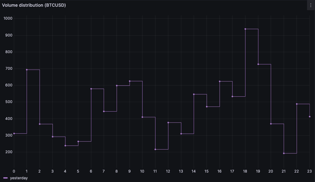
For example, you could calculate the hourly average volumes from yesterday, and the past week or month to identify high-liquidity periods. As a simple example, we could go with the assumption that today's volume should be distributed similarly to yesterday's.
We can derive yesterday's volume profile as follows:
WITH x AS
  (
    SELECT timestamp, sum(amount) qty
    FROM trades
    WHERE symbol = 'BTC-USD'
      AND timestamp > dateadd('d', -1, now())
    SAMPLE BY 1h
    ALIGN TO CALENDAR
  )
SELECT hour(timestamp), qty yesterday
FROM x ORDER BY hour ASC
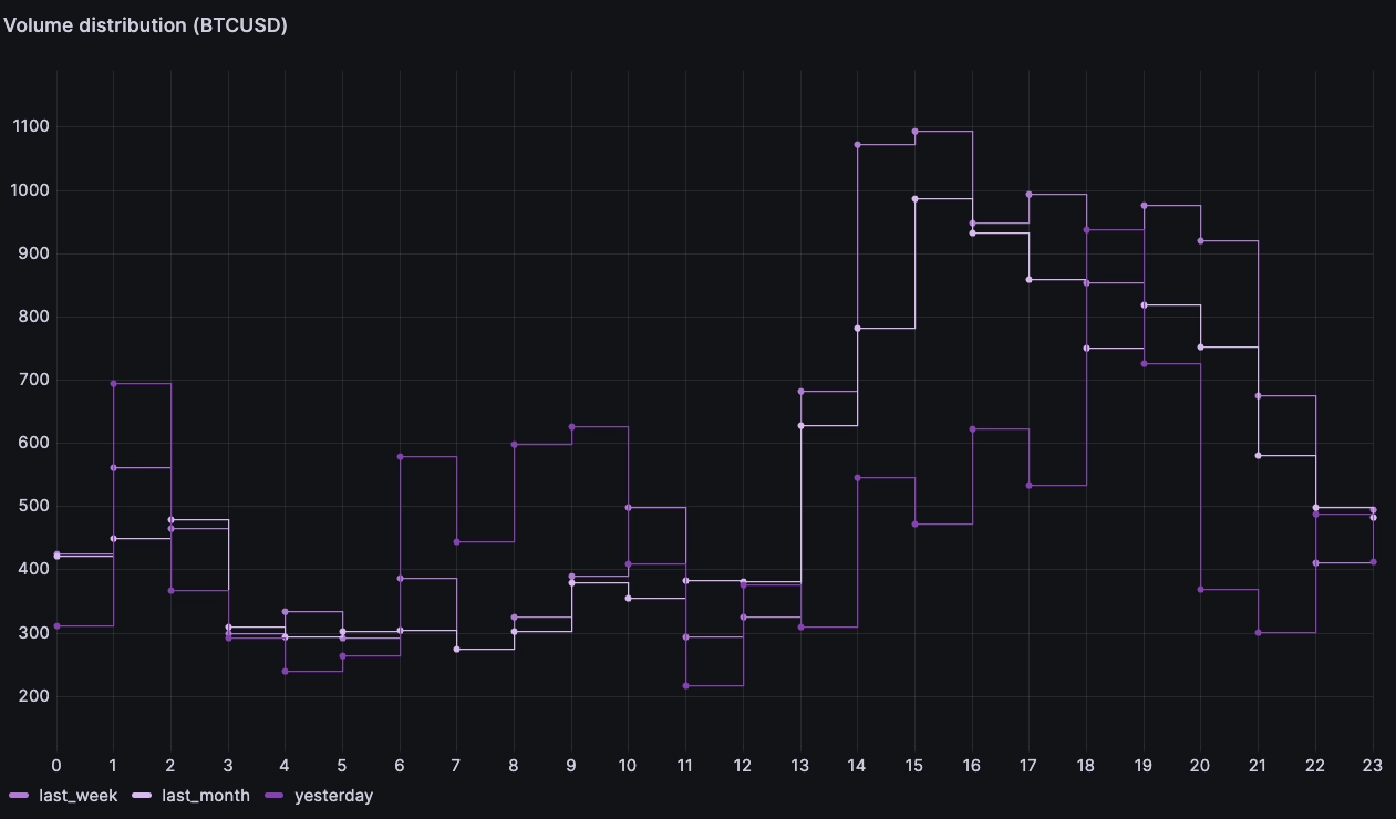
We can then expand on this and compare it to other dates or intervals. For
example, we can compare with the average over the last week or month by adding
an avg() function and changing the lookback period:
WITH x AS
  (
    SELECT timestamp, sum(amount) qty
    FROM trades
    WHERE symbol = 'BTC-USD'
      AND timestamp > dateadd('d', -30, now())
    SAMPLE BY 1h
    ALIGN TO CALENDAR
  )
SELECT hour(timestamp), avg(qty) last_month
FROM x
ORDER BY hour ASC
Using this data, the trading strategy can estimate when liquidity is expected to be high, and slice large orders accordingly.
Synthesizing volume predictions
There is a lot of science in making a volume prediction. But a simple approach could be to use different lookback intervals with different weights assigned to different periods.
For example, one approach would be to favour stability, and assign more weight to the longer lookback, and less weight to the more recent lookback. This approach means we account for recent changes in liquidity, but do not overly shift our distribution if there was an abrupt change recently which we believe is transient.
Using the example above, we could combine queries to synthesize a volume distribution with the following weights:
- 50% monthly lookback
- 30% weekly lookback
- 20% yesterday
WITH
  yest as (
    WITH x AS (
      SELECT timestamp, sum(amount) qty
      FROM trades
      WHERE symbol = 'BTC-USD'
        AND timestamp > dateadd('d', -1, now())
      SAMPLE BY 1h ALIGN TO CALENDAR
    )
    SELECT hour(timestamp) h, qty daily
      FROM x ORDER BY h asc
  ),
  week as (
    WITH x AS (
      SELECT timestamp, sum(amount) qty
      FROM trades
      WHERE symbol = 'BTC-USD'
        AND timestamp > dateadd('d', -7, now())
      SAMPLE BY 1h ALIGN TO CALENDAR
    )
    SELECT hour(timestamp) h, avg(qty) weekly
      FROM x ORDER BY h asc
  ),
  mth as (
    WITH x AS (
      SELECT timestamp, sum(amount) qty
      FROM trades
      WHERE symbol = 'BTC-USD'
        AND timestamp > dateadd('d', -30, now()    )
      SAMPLE BY 1h ALIGN TO CALENDAR
    )
    SELECT hour(timestamp) h, avg(qty) monthly
      FROM x ORDER BY h asc
  )
SELECT
  mth.h as hour,
  0.5*monthly + 0.3*weekly + 0.2*daily as volume
FROM yest join week on yest.h = week.h
          join mth on mth.h = yest.h
ORDER BY h ASC
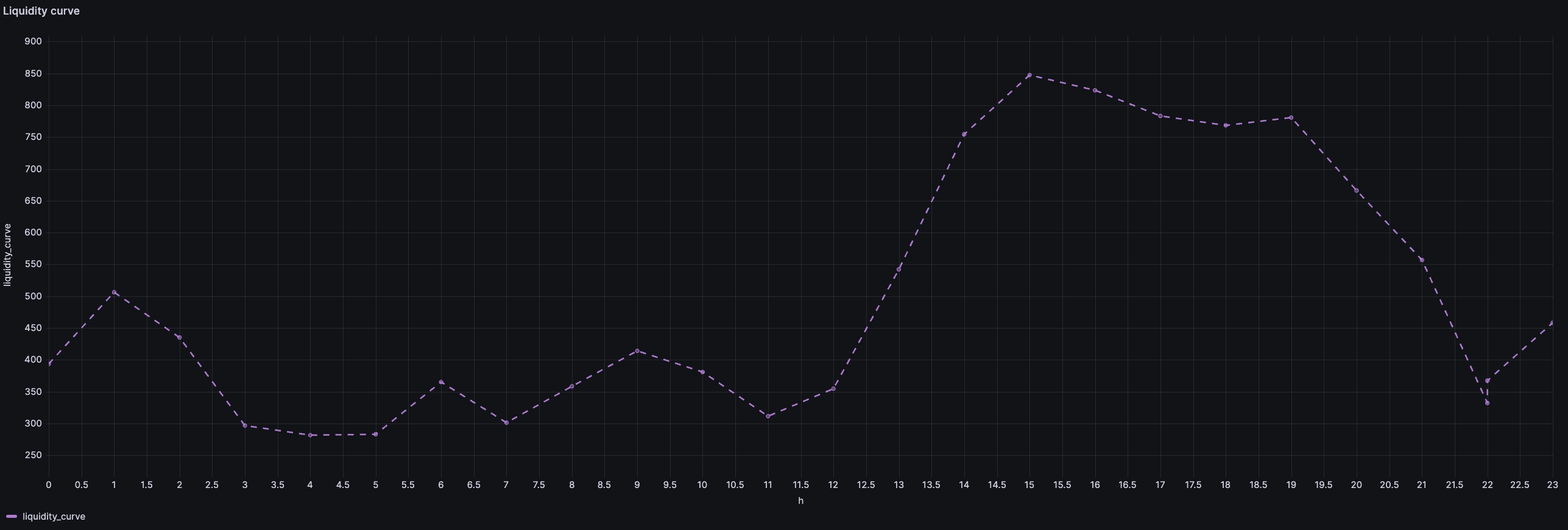
The output can then be used as a volume profile for slicing VWAP orders over the planned execution period. For example, an order executed throughout the full day would have fewer executions in the morning, and ramp up the pace in the afternoon.
Demonstration of slicing
Let's say we want to buy 100 BTC between 10am and 3pm, and want to achieve a price close to the VWAP over that period. The historical curve we just derived shows the following volume distribution:
| Hour | BTC | Pct |
|---|---|---|
| 10 | 391 | 12.3% |
| 11 | 352 | 11% |
| 12 | 382 | 12% |
| 13 | 498 | 15.3% |
| 14 | 716 | 22.4% |
| 15 | 854 | 26.7% |
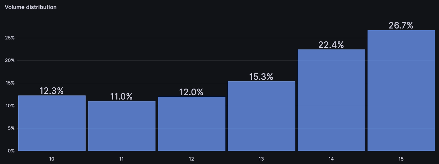
Based on this, our algo could slice our 100BTC order such that it would execute 12.3BTC between 10 and 11, 11BTC between 11am and noon, and so on... While this example is simple, we may want to take a few elements into consideration before sending an order out.
Other important considerations
The example above comes up with a strategy to execute X BTC in a set of one-hour windows. However, we still need to consider how to execute within each hour.
If we execute each 1-hour chunk in one go, we risk distorting the market and getting a less favourable execution price. In addition, our execution will be skewed towards the prevailing price at the moment of execution. If the price moves significantly, the resulting VWAPs from executing at the beginning, middle, and end of the hour could be vastly different.
We could mitigate this by simply increasing the resolution of our VWAP liquidity curve, using an interpolation function between the hourly percentages, or deriving a curve with greater resolution, such as 10-minute intervals.
Another option is to keep the hourly intervals, but use a TWAP strategy with some level of price and time randomization to trade the required quantity within the hour. Randomization and mixing of different strategies is generally a good idea. It makes it harder for other market participants to identify trading patterns and discover hidden liquidity in the market. As a consequence, this improves our execution price.
Another important consideration is the relative size of the order. If your order is large compared to the ordinary volume, then a significant part of the trading volume over the target VWAP period will be yours.
Intuitively, this means that you are more likely to get an average execution price close to the actual VWAP. However, it could also mean you will hit poor liquidity if your order outsizes what the market can take.
So while the final execution price would be close to the VWAP, it may also incur large trading costs compared to executing the VWAP over a larger time window. Depending on the liquidity, trading a certain quantity via VWAP over a certain period may not be viable.
Conclusion
VWAP is one of the most important financial execution algorithms. Calibrating and fine-tuning them is a complex piece of work, which balances historical data and realtime on-the-fly adjustments. While this article is not meant to be exhaustive, it should help you build intuition for how a VWAP algo works behind the scenes.
Come talk to us on Slack or Discourse!