How to generate time-series data in QuestDB

This post comes from Gábor Boros, who has written an excellent tutorial that shows how to mock timeseries data using built-in SQL functions in QuestDB to generate dummy data for testing and rapid prototyping according to custom schemas. Thanks for the submission, Gábor!
Mocking and generating time series data
As developers, we often have to generate sample data for numerous reasons: feeding integration tests, realistic staging environments or developing an application locally.
This process can be time-consuming, especially when we need data on a bigger scale. Fortunately, some databases are helping our work and trying to offload some weight from our shoulders by providing functions to generate data.
This tutorial will cover how to generate test data using QuestDB using built-in generators so you can quickly mock data similar to your own production data.
Types of time series data
Before diving deep into generating data using QuestDB, we need to take one step back to discuss what types of time series data we can generate, what "mock data" is, and what generator functions are available for use. Let's start with the different types of time series data. We can classify the data based on the frequency we receive them into two categories: regular and irregular data.
Regular data is received per a pre-defined period, usually collected by a collector node or sent by an agent. Collecting metrics from a server fits into this category perfectly, as shown in the tutorial where we connected Telegraf with QuestDB. The Telegraf agent running on the server collects the metrics on a pre-defined basis and sends them to the QuestDB instance.
The opposite of regular data is the irregular data which is collected dynamically. The main point about irregular data is that we cannot predict how often the data will arrive. As of examples, automating ETL jobs could be a great example. The data comes in when automation or the user sends it to the pipeline, hence we cannot know beforehand the data arrives.
Of course, these categories can split into multiple groups, for instance, based on the field it used: IoT, financial, operations, industrial telemetry, and so on. Regardless of how we categorize the data, the most important is knowing the data and use-case before generating it.
What is mocking and why is it useful?
Software development is about making things, but in some cases, testing what we make is challenging. There are multiple scenarios when we want to check for errors and failures, invalid input, we need lots of test data, or we want to operate a production-like environment without user data.
The function or application we test may have dependencies. To test the edge cases, we have to isolate and simulate the behavior of these dependencies. This kind of simulation can happen on multiple levels. Think about integration test suites; we do not want to imitate the behavior of the components we are testing, but we may want to load fake data in the system.
Simulation of the behavior of components or data is called mocking. Remember the ETL job mentioned above. If we would like to test hundreds of thousands of processing, we would need to craft the input data on our own. That would be time-consuming and ineffective. On the other hand, generating mock data help us focus on the processor job, not the data generation.
The way we generate mock data may differ case-by-case. Since it highly depends on the application being developed, let's see how can we mock different types of data with QuestDB easily.
Running QuestDB
To discover the capabilities of how QuestDB can generate data for us, we need to run it. We will use Docker and the latest questdb Docker image for convenience. To start QuestDB via Docker, run the following:
docker run -p 9000:9000 \-p 9009:9009 \-p 8812:8812 \questdb/questdb
Alternatively, macOS users can use Homebrew:
brew install questdbbrew services start questdb
The QuestDB downloads page has downloads for binaries if you wish to run it as a standalone.
Mocking different types of data in QuestDB
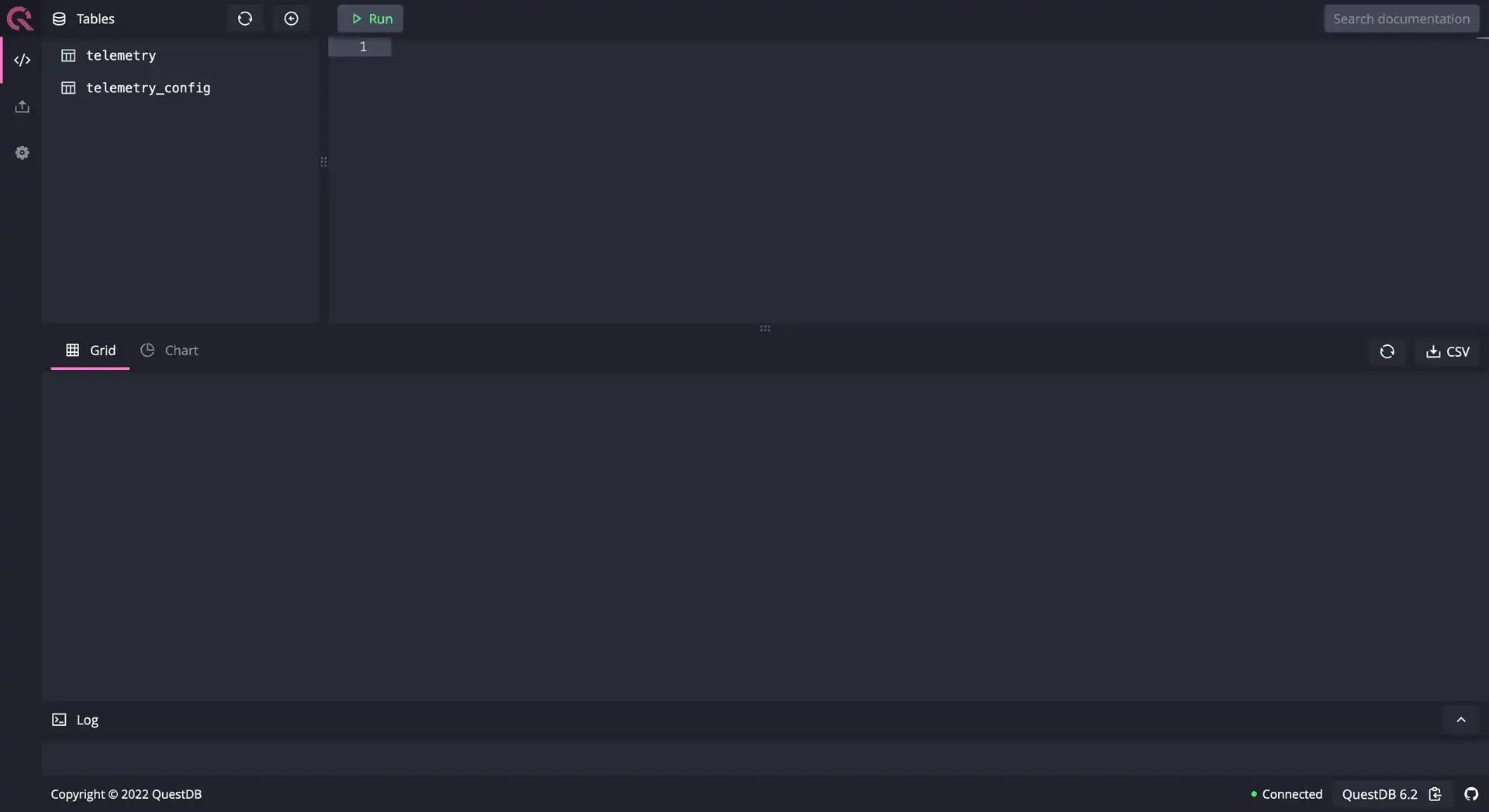
After starting QuestDB, the Web Console is available on
port 9000, so navigating to http://127.0.0.1:9000 should show the UI of a
locally-running instance which looks like the following:
Mock data generation in QuestDB is surprisingly easy. The DB comes with numerous
generator functions, all with a different purpose. If you ever used PostgreSQL's
generate_series, you will find QuestDB's generator functions pleasant and
relieving. To generate rows, we use the
long_sequence
generator function that can create billions of rows depending on our needs. Its
syntax looks like
SELECT <COLUMNS> FROM long_sequence(<NUMBER_OF_ROWS>[, <SEED1>, <SEED2>]]);
If we need deterministic row generation, we can optionally provide <SEED1> and
<SEED2>, that are 64 bit integers, and anchor the start of the random
generator to obtain the same sequence on every run. That could be useful when
populating data for tests, CI/CD pipelines, or development environments. Let's
generate some rows to see long_sequence in action.
For a first query, paste the following in the SQL editor:
SELECT x, x*x FROM long_sequence(5);
You will see five rows with two columns. The first column counts from one to five, while the second column contains the square of the values of column one.
| x | column |
|---|---|
| 1 | 1 |
| 2 | 4 |
| 3 | 9 |
| 4 | 16 |
| 5 | 25 |
Easy, right? It is that simple to get started on generating mock data with QuestDB. We have basic example of generating numbers, and next, we'll look at generating booleans, characters, strings, timestamps, and many more types.
Generator functions in QuestDB
We have seen how to generate basic rows, and we mentioned random value generation too. It's time to see how we can generate random values with QuestDB's built-in random generator functions.
QuestDB supports random generator functions for several data types:
| type | generator function |
|---|---|
| binary | rnd_bin |
| boolean | rnd_boolean |
| byte | rnd_byte |
| char | rnd_char |
| date | rnd_date |
| double | rnd_double |
| float | rnd_float |
| geohash | rnd_geohash |
| int | rnd_int |
| long256 | rnd_long256 |
| long | rnd_long |
| short | rnd_short |
| string | rnd_str |
| symbol | rnd_symbol |
| timestamp | rnd_timestamp |
All these functions can be parameterized with seed values to narrow the function's range. This is an extremely useful feature, especially if we need to debug our application using the generated test data.
Although these functions can be handy in many scenarios, it is important to highlight that these functions should be used for populating test tables only. They do not hold values in memory and calculations should not be performed at the same time as the random numbers are generated.
The best practice when populating test tables is creating the table first, then populating and querying it. Consider the following example:
SELECT round(a,2), a FROM (SELECT rnd_double() a FROM long_sequence(10));
This would return inconsistent and ephemeral results while the approach below will return consistent results that are persisted as a normal database table.
-- creating the table firstCREATE TABLE test(val double);-- populating the test tableINSERT INTO test SELECT * FROM (SELECT rnd_double() FROM long_sequence(10));-- querying generated dataSELECT round(val,2) FROM test;
Now that we know what types of data can be generated and have seen how to generate random values, it is time to create more complex data.
Creating realistic generative data
To see data generation in action, we will replicate the schema used by the Time Series Benchmark Suite, a tool for comparing and evaluating databases for time series data.
In the benchmarking example, TSBS uses truck diagnostic data sent through the InfluxDB protocol to populate tables. We will take a different approach. Instead of sending the data, we will generate it directly using the web UI.
Following the approach described above, let's create the table first. Navigate
to the web UI and create the diagnostics table that you can see below.
CREATE TABLE 'diagnostics' (name STRING, -- identifier of the truckfleet STRING, -- division where the truck belongs todriver STRING, -- the name of the driver who drove the track on the given daymodel STRING, -- the model of the truckdevice_version STRING, -- version number of the data collector deviceload_capacity INT, -- maximum load capacity of the truck at the beginning of the shiftfuel_capacity INT, -- fuel capacity of the truck at the beginning of the shiftnominal_fuel_consumption INT, -- fuel consumption at the given timefuel_state DOUBLE, -- the current state of the fuel level: 1 is full, 0 is emptycurrent_load INT, -- the weight of the current loadstatus INT, -- status of the truckts TIMESTAMP -- timestamp the diagnostic entry got recorded) timestamp(ts) PARTITION BY year;
By this point, we have the table without any records. For now, we don't set constraints on the data, like the capacity must be consistent or fuel capacity should remain the same over the days. Also, we assume that we get a report from a sensor per hour, no matter from which truck.
Keeping the above in mind, let's populate the table with some test data. For
doing that, we are going to use four different random value generators, namely
rnd_int, rnd_double, rnd_str, and rnd_timestamp. All these functions
have different arguments and capabilities. To generate some rows, run the
following query:
INSERT INTO 'diagnostics' SELECT * FROM (SELECTrnd_str('truck_1234', 'truck_5678', 'truck_9123', 'truck_3210'),rnd_str('North', 'East', 'South', 'West'),rnd_str('Alice', 'Bob', 'John', 'Mike', 'Robert'),rnd_str('G-0', 'H-2', 'I-1'),rnd_str('v1.2', 'v1.3'),rnd_int(1000, 1500, 0),rnd_int(150, 200, 0),rnd_int(0, 15, 0),rnd_double(),rnd_int(0, 1500, 0),rnd_int(0, 4, 0),rnd_timestamp(to_timestamp('2022-01-01T00:00:00', 'yyyy-mm-ddTHH:mm:ss'),to_timestamp('2022-02-28T23:00:00', 'yyyy-mm-ddTHH:mm:ss'),0)FROM long_sequence(28));
After the query ran successfully, ensure we have the 28 records we expect. Run
SELECT * FROM 'diagnostics';
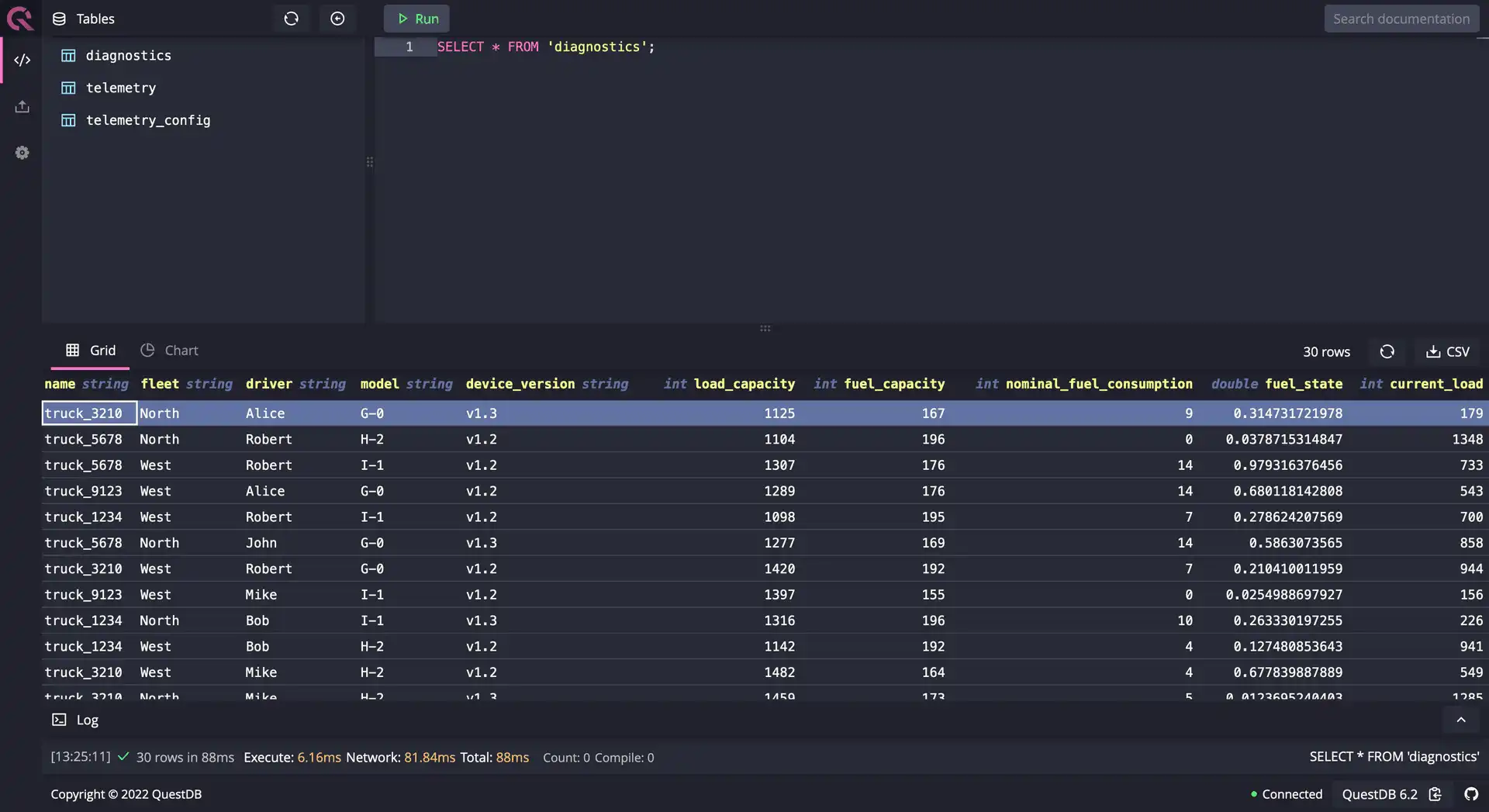
Congratulations, we successfully generated twenty eight rows with random data.
Although the data is in place, the timestamps seem to be odd; we have multiple
records for the same hour. The reason behind this is how rnd_timestamp works.
It generates data within the given range, without considering any sequence.
To fix this issue, we need to use a timestamp sequence generator, called
timestamp_sequence. This generator can be used as a timestamp generator to
create data for testing. The timestamp is increased by providing a steps
argument, which sets the step size in microseconds.
SELECTtimestamp_sequence(to_timestamp('2022-02-01T00:00:00', 'yyyy-mm-ddTHH:mm:ss'),3600000000L)FROM long_sequence(10);
Running the query above generates ten rows, where every row will follow the previous row's value increased by one hour.
Now that we know how we can generate sequentially increasing timestamps,
refactor the query we used to generate test data as follows. Before running the
query, execute truncate table 'diagnostics' to clean up the previously
generated rows.
INSERT INTO 'diagnostics' SELECT * FROM (SELECTrnd_str('truck_1234', 'truck_5678', 'truck_9123', 'truck_3210'),rnd_str('North', 'East', 'South', 'West'),rnd_str('Alice', 'Bob', 'John', 'Mike', 'Robert'),rnd_str('G-0', 'H-2', 'I-1'),rnd_str('v1.2', 'v1.3'),rnd_int(1000, 1500, 0),rnd_int(150, 200, 0),rnd_int(0, 15, 0),rnd_double(),rnd_int(0, 1500, 0),rnd_int(0, 4, 0),timestamp_sequence(to_timestamp('2022-01-01T00:00:00', 'yyyy-mm-ddTHH:mm:ss'),3600000000L)FROM long_sequence(28));
The new query will create 28 records, where all timestamps increase by one hour.
Although this is close to what we would like to see, it is still not 28 days.
From now on, we need to do some basic math. To get 28 days of records where
every record is one hour away from the previous one, we need to generate
28 * 24 records (that's 672 records).
Changing FROM long_sequence(28) to FROM long_sequence(672) and running the
query will generate the expected number of records with the expected timestamp
differences.
So far, we have learned how to generate simple and more complex test data, also we experienced the difference between generating random timestamps and sequentially increasing timestamps. You may now wonder, "How could we generate ten years of data?". The answer is simple, and you probably assume it: let's calculate a bit.
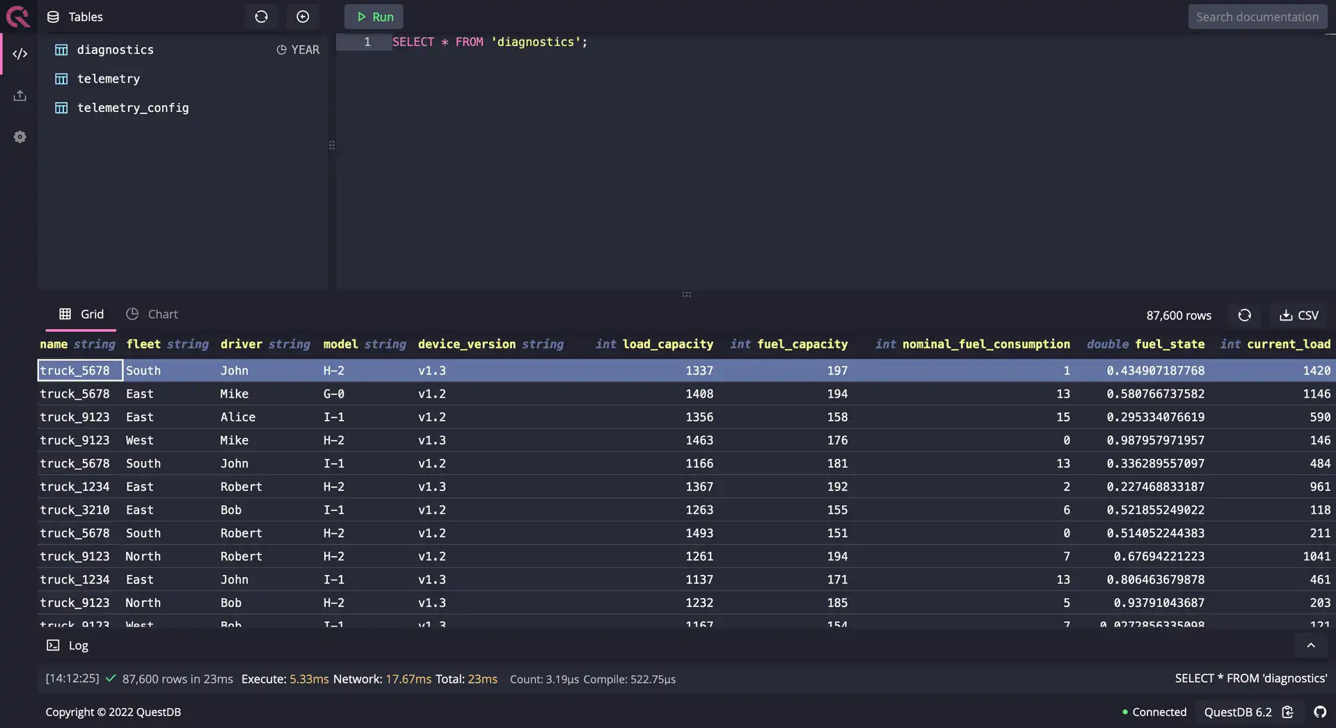
If we would like to generate test data for one year, we would need to generate
365 * 24 records. Based on this logic, to produce the desired ten years of
random data we generate 10 * 365 * 24 records, which is 87600 rows. By simply
changing the long_sequence parameters to 87600 and running the query one
more time, we can generate data for the next ten years in less than a second.
Summary
In this tutorial, we discussed what mock data is useful, what kinds of types are available in QuestDB, how to generate random data, and create tables with test data for 1, 3, or 10 years. This tutorial demonstrated well how to combine the generator functions to create complex generative data. Thanks for your attention!
If you like this content, we'd love to know your thoughts. Feel free to share your feedback or just come and say hello in the community forums.