Time-series and analytical databases walk into a bar

The following write-up is based on a talk from P99 CONF 2024.

Watch the talk and/or read along!

Presented by: Andrei Pechkurov, Core Engineer at QuestDB

Introducing Andrei and QuestDB​

Hello everyone! Today, I'll be discussing the differences between time-series databases and analytical databases and how we improved our time-series database at QuestDB to handle both efficiently. Many of the techniques and optimizations I'll cover are relevant to modern databases, making this talk helpful for anyone interested in analytical database performance.

But first, let me introduce myself. I'm Andrei Pechkurov, part of the QuestDB core engineering team. I have a passion for concurrency, performance, and distributed systems, and when I'm not working on the QuestDB query engine with our amazing team, you'll find me enjoying board games with my family.

Time-Series vs. analytical databases​

Before diving into the specifics, let's get a clear picture of the differences between time-series databases and analytical databases. For storytelling purposes, I'll be using QuestDB as an example of a time-series database.

Meet QuestDB​

QuestDB is an open-source time-series database licensed under Apache 2.0. It supports SQL with specialized extensions for time-series data and provides high-speed ingestion via InfluxDB's line protocol over TCP or HTTP. The data is stored in a columnar format, partitioned and ordered by time, and can be native or Parquet.

QuestDB is written mostly in Java, with portions in C++ and Rust. It features optimizations inspired by high-frequency trading systems, including zero garbage collection (GC) on the hot path and the use of an in-house API instead of Java's standard library. Our parallel, vectorized query engine also comes equipped with a JIT compiler.

Time-series database specifics​

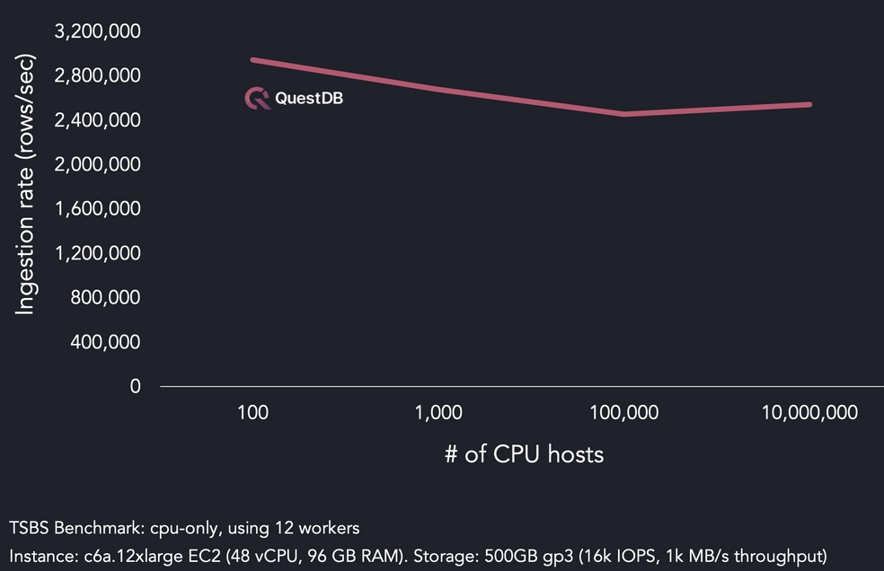
The primary strength of a time-series database is its ability to handle intensive data ingestion, with rates reaching up to several million rows per second on a single server. This is crucial for real-time applications, where the database must quickly process and store new data.

Querying nascent data​

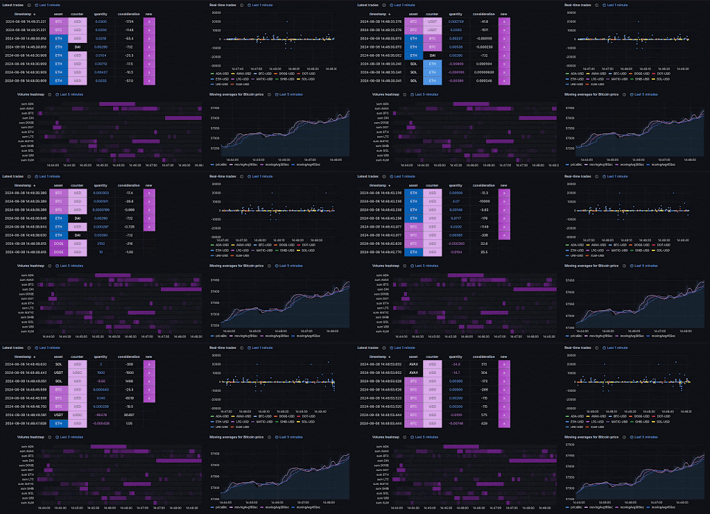
One key aspect of time-series databases is that they typically process nascent data—the most recent data that's often displayed on dashboards or used for immediate analysis. In fields like trading which process tick data, this might represent data from just the past few minutes:

SQL extensions for time-series data​

Time-series databases often provide SQL extensions to make querying recent data easier. In QuestDB, for example, we have the SAMPLE BY syntax for aggregating data over time intervals and LATEST ON to fetch the latest values for each time-series. This allows users to efficiently analyze fast-changing datasets. Let's test them out.

Click the demo link on any of the following queries to run them within our live demo:

SELECT pickup_datetime, count()
FROM trips
WHERE pickup_datetime IN '2018-06-01;7d'
SAMPLE BY 1h FILL(NULL);

SELECT
  pickup_datetime,
  fare_amount,
  tempF,
  windDir
FROM (
  SELECT * FROM trips
  WHERE pickup_datetime IN '2018-06-01'
) ASOF JOIN weather;

SELECT *
FROM trades
WHERE symbol IN ('BTC-USD', 'ETH-USD')
LATEST ON timestamp PARTITION BY symbol;

SELECT
  timestamp,
  vwap(price, amount) AS vwap_price,
  sum(amount) AS volume
FROM trades
WHERE
  symbol = 'BTC-USD'
  AND timestamp > dateadd('d', -1, now())
SAMPLE BY 15m ALIGN TO CALENDAR;

Analytical database features​

While time-series databases excel at real-time ingestion and queries, analytical databases have their own set of strengths. They usually support complex queries like GROUP BY, JOIN, and filters that process large datasets, not necessarily accessed over time.

Analytical databases also typically leverage multi-threading and use columnar storage formats to optimize query performance. These databases are built to handle deep, non-time-based analytical queries, often running over massive datasets.

A time-series database is an analytical database​

At this point, you might be thinking, "Aren't time-series databases just a form of analytical database?" And you'd be right!

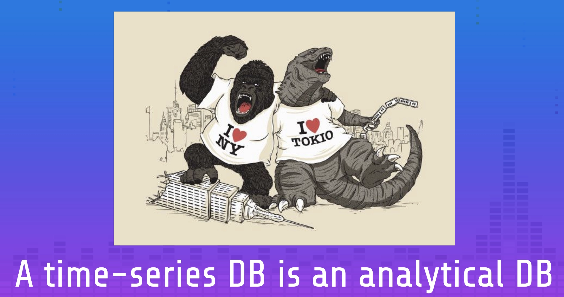
However, a couple of years ago we noticed that some of our QuestDB users were running analytical queries, but they weren't satisfied with the performance. So, we decided to improve QuestDB's analytical capabilities.

How to improve analytical database performance​

To improve analytical performance, we began by focusing on existing benchmarks, such as:

• ClickBench – A benchmark created by the ClickHouse team in 2022, focusing on complex queries like GROUP BY, WHERE, and ORDER BY.
• db-benchmark by DuckDB Labs
• TPC Benchmarks
• TSBS (Time Series Benchmark Suite)

Our first focus was on ClickBench, where we saw opportunities for optimization. Initially, our results were disappointing:

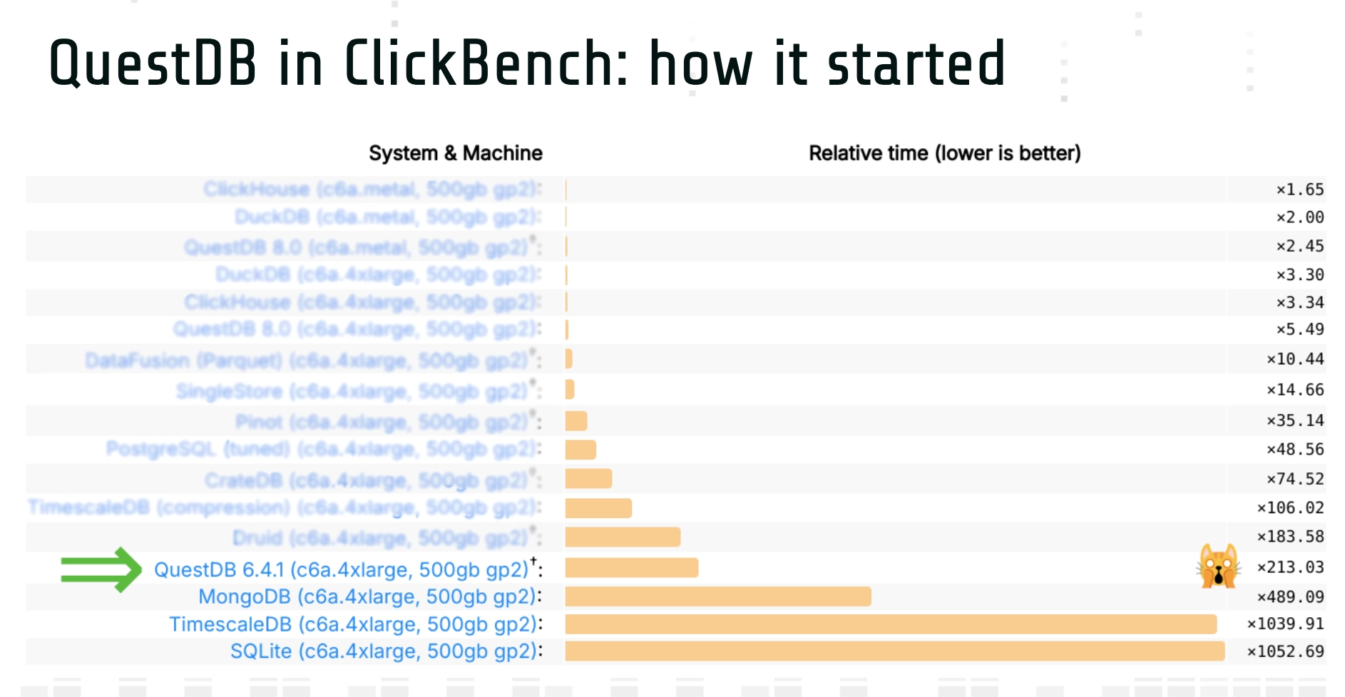
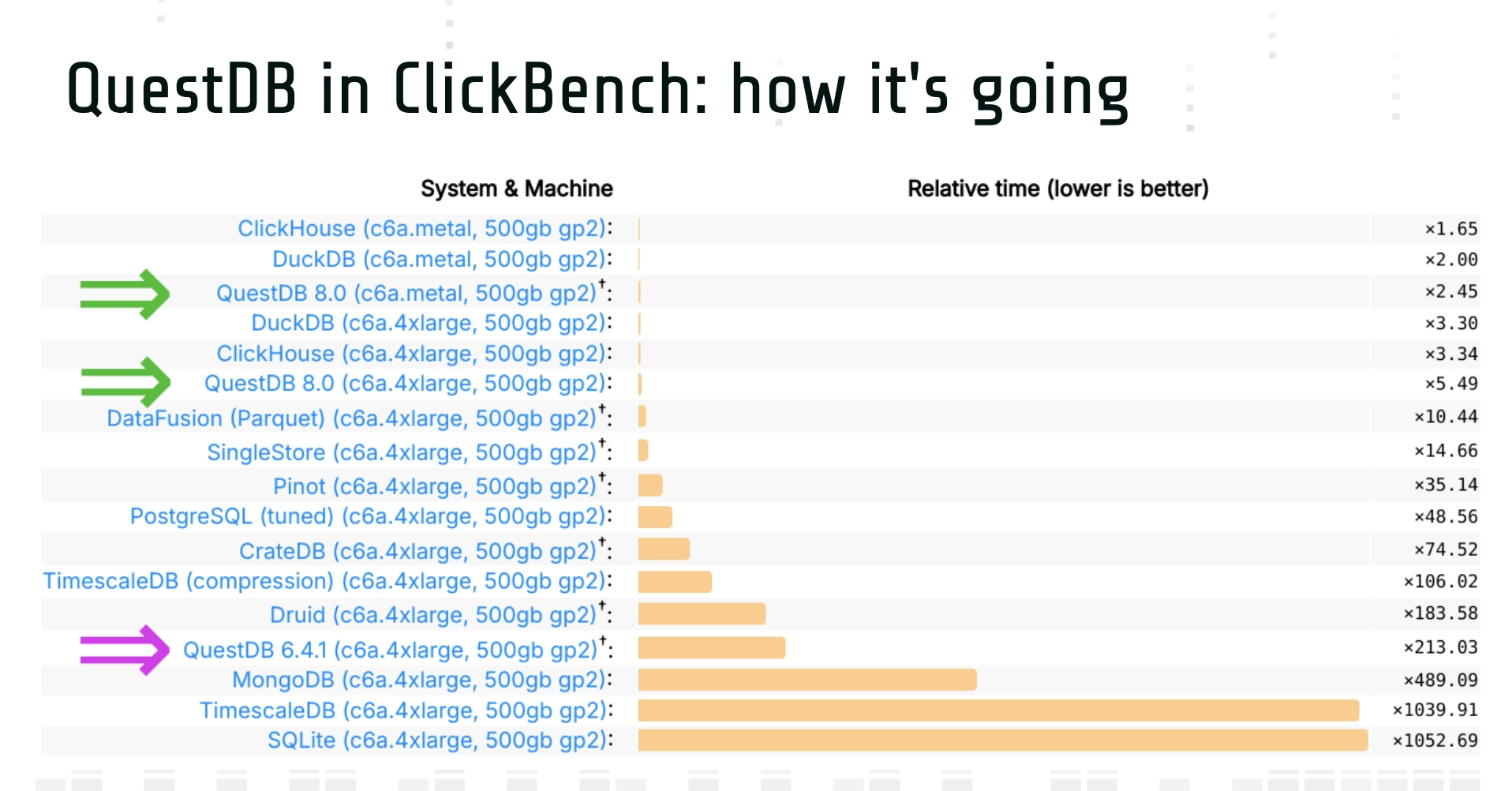
Luckily, after two years of work—alongside developing major features like Write-Ahead-Log (WAL) and replication—we made massive improvements, jumping two orders of magnitude in performance.

The journey to optimization​

Improving QuestDB's analytical capabilities took time—two years to be exact. Along the way, we implemented around 80 patches, some contributed by our community, and overcame several failed optimization attempts. The journey was full of valuable lessons and led to exciting improvements in the database's performance:

Key improvements​

Here are some of the trivial but impactful changes we made:

• Added missing SQL functions like count_distinct() for integer columns and improved memory efficiency for others to avoid crashes.
• Expanded our SQL JIT compiler for WHERE clause filters, supporting more operators and types, which sped up queries involving filters.
• Optimized SQL functions like the LIKE operator, vectorizing it for short ASCII patterns to reduce overhead.

Specialized hash tables​

One key innovation was introducing specialized hash tables for parallel aggregation. These tables support small fixed-size keys like 32-bit and 64-bit integers, as well as single VARCHAR keys, making GROUP BY operations significantly faster.

Check out this blog post to learn more about design decisions behind one of our hash tables.

Lessons learned​

Through this journey, we learned that:

1. A fast time-series database must also be capable of running analytical queries.
2. Benchmarks like ClickBench can be useful starting points, but real-world workloads must guide the optimization process.
3. Improving the efficiency of a query engine requires planning and discipline. The impact of these optimizations was significant, and we even managed to parallelize SAMPLE BY queries in the process.

Deep dive: Parallelized SAMPLE BY queries​

Our version one had some good things going for it:

• Simple pipeline, easy to implement
• Scales nicely when there are not so many groups (distinct UserID values)
• Yet, high cardinality (>= 100K groups) is a problem

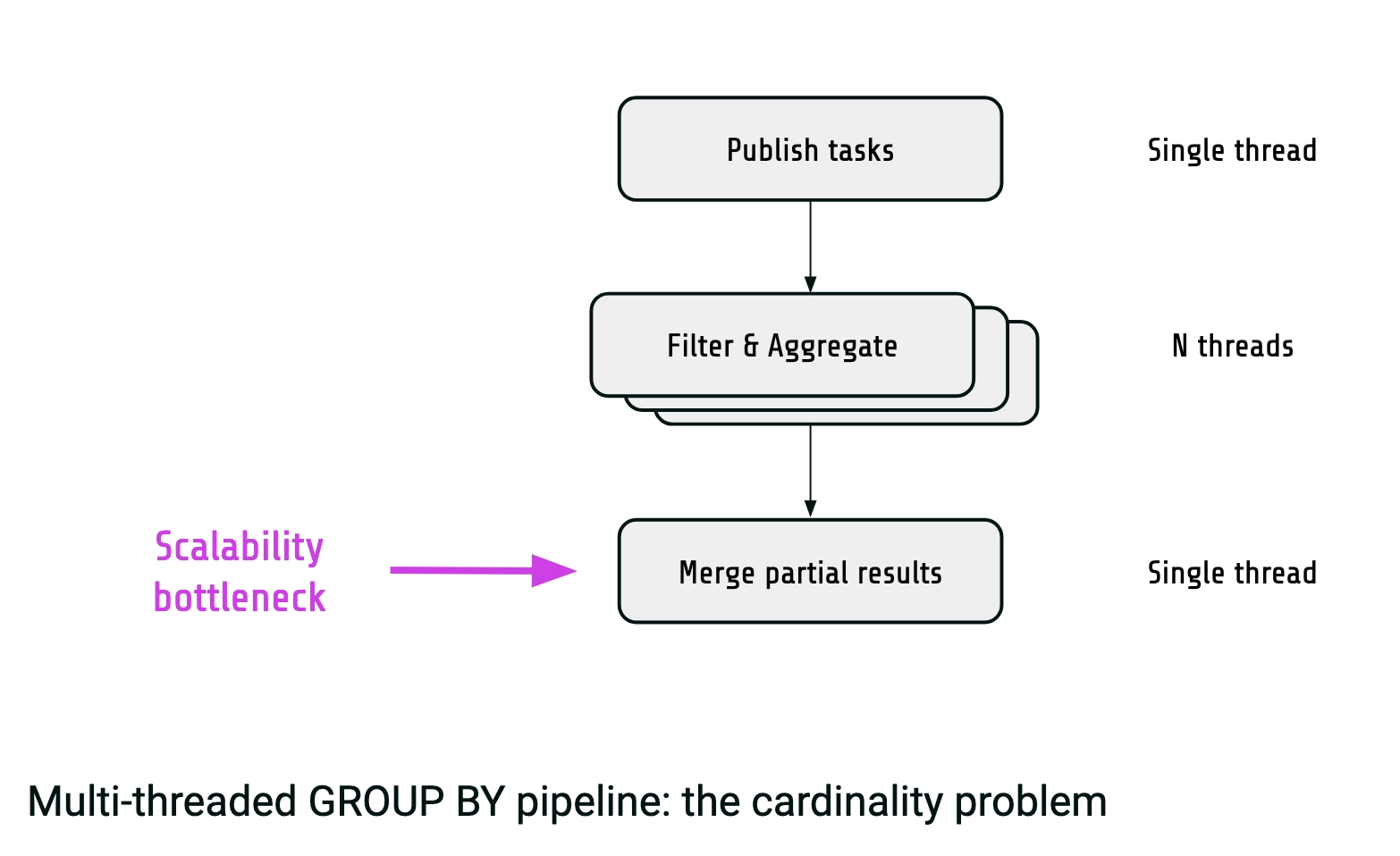
The merge step is the bottleneck. With so many groups it becomes too slow and simply eliminates the speed up from the previous parallel step. Luckily, it's possible to improve the pipeline for the high cardinality scenario.

Radix-partitioning​

We can use radix-partitioning:

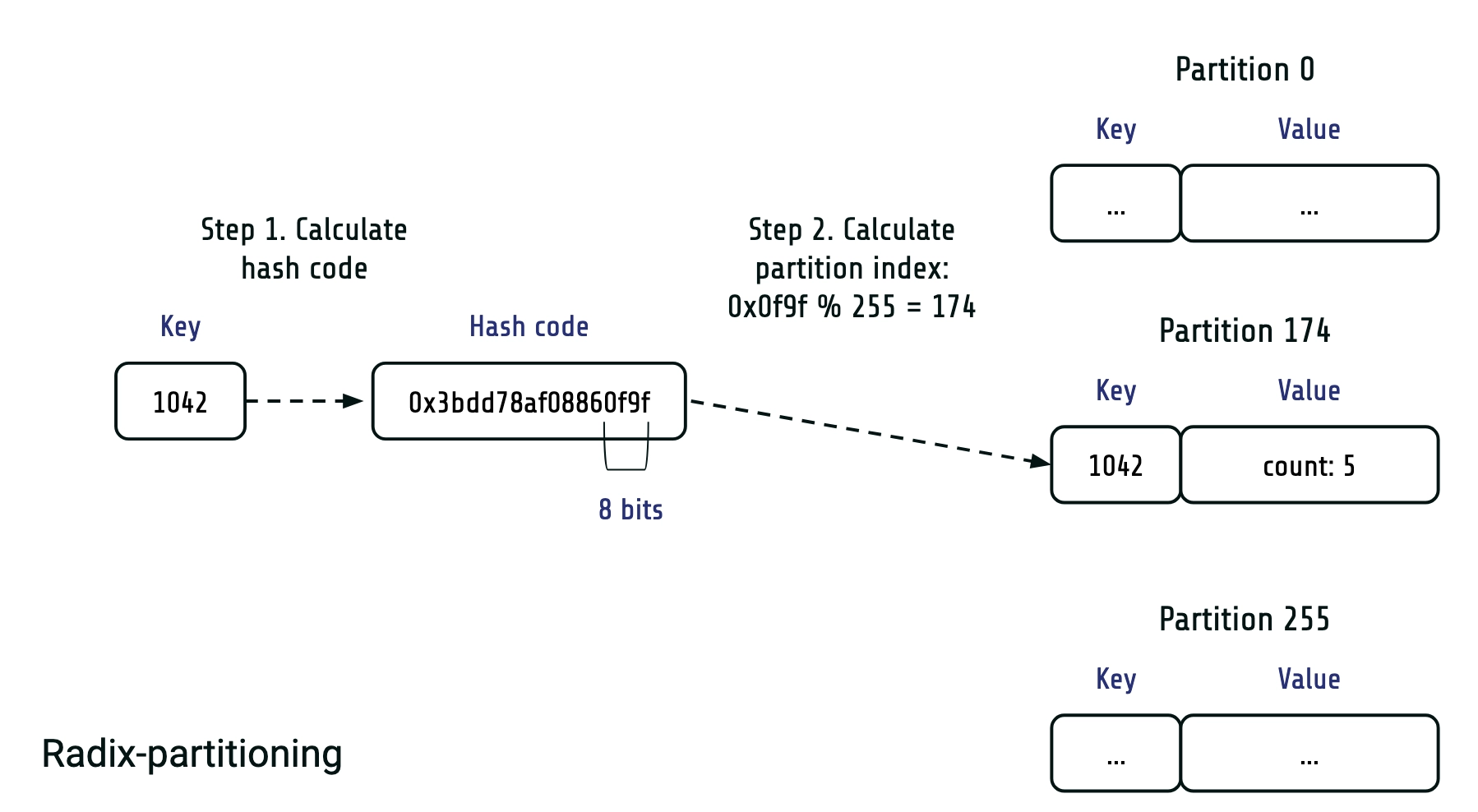
It can be met in parallel hash join algorithms, but is also applicable to GROUP BY. The idea is simple: we divide all scanned rows into multiple partitions, based on a few bits of the group hash code. For example, if we use lowest 8 bits of the hash code we'll have 256 partitions. Potentially radix-partitioning is prone to skew due to unlucky combination of keys and hash function, but in real world the probability of this is very small.

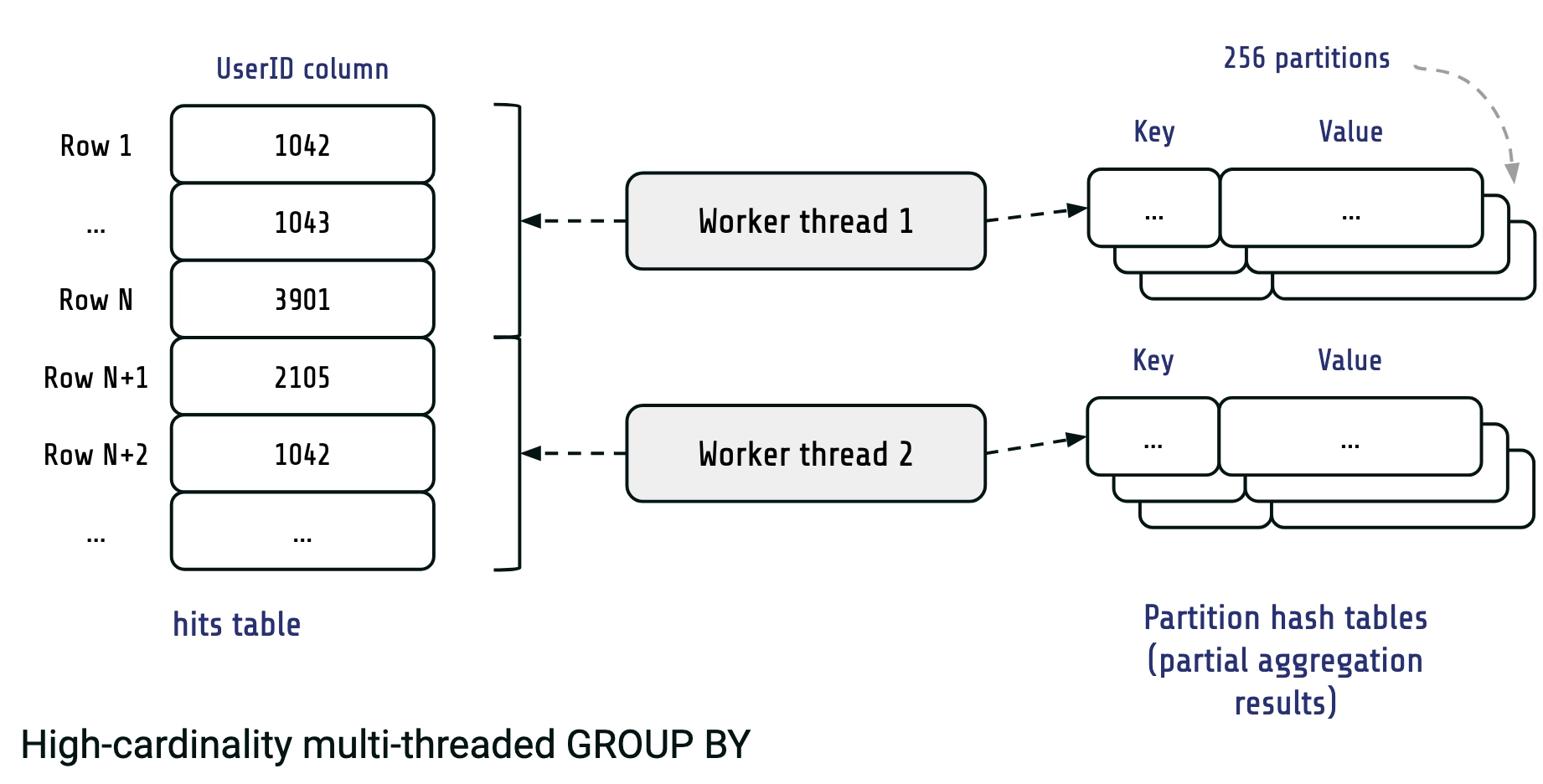
Getting to V2​

With radix partitioning, our worker threads produce a number of hash tables. Each of these hash tables corresponds to a partition. Thus, in our example partial results consist of 256 hash tables instead of a single one. Each of the partitions contains isolated subsets of the final result, so we can merge them independently and in parallel.

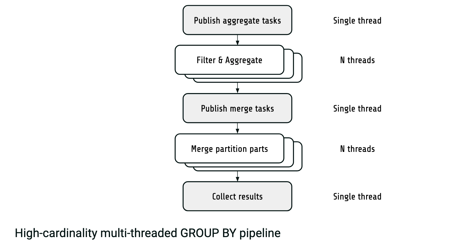
In the high-cardinality case, our improved pipeline now looks like this:

End result​

It involves a new parallel merge step. Once we've got partial aggregation results, we publish a merge task for each radix partition, so that they're merged in parallel. This way we get rid of the single-threaded merge bottleneck.

• More complex pipeline, a bit harder to implement
• Scales nicely for any cardinality
• Potentially parallel ORDER BY + LIMIT when the cardinality is high
• Used for multi-threaded GROUP BY and SAMPLE BY

SELECT pickup_datetime, count()
FROM trips
WHERE pickup_datetime IN '2018-06-01;7d'
SAMPLE BY 1h;

The road ahead​

Looking ahead, we plan to continue improving QuestDB's analytical performance. We've already made progress by implementing parallel GROUP BY pipelines as shown above, and we're now working on further optimizations, particularly for high cardinality queries.

Conclusion​

Thank you for reading/watching my talk today. If you'd like to learn more about QuestDB or have any questions, feel free to reach out!

To learn more about QuestDB, check out our GitHub repository, try the demo, or join the conversation on Slack.