Revealing the stories in French real estate data
Real estate markets have been all over the place since COVID.
In countries such as the UK where mortgage rates are indexed to the central bank, it seems harder for many to meet increased mortgage payments and harder to sell or remortgage property. In the US, while most mortgages are fixed-rate, rising interest rates still squeeze new buyers and those looking to refinance, making affordability a growing concern.
In urban centres, generalised work-from-home policies reduced the need for office space and the profitability of commercial landlords. We also heard of an exodus from cities to suburbs following the lockdowns.
But what's really happening? Does the underlying data confirm these stories, or unveil new ones? We'll look into France because of a personal connection and residual Olympic enthusiasm.
Bon voyage!
Our real estate dataset
The Demande de Valeurs Foncières (DVF) is a publicly accessible dataset provided by the French government. It's based on notary records and contains information about real estate transactions in France, allowing individuals, researchers, and professionals to access detailed property data. It includes information on the date of the transaction, the sale price, surface and property details.
Enriched versions such as this one are also available and include additional information such as the coordinates of the parcel which will further allow us to visualise the data on a map:
Index of /geo-dvf/latest/csv/
../
2019/
2020/
2021/
2022/
2023/
2024/
Follow along
To reproduce and follow the examples in this tutorial, you'll need:
- A running instance of QuestDB
- Not running yet? Check out the quick start.
- A running instance of Grafana
- We've got a small guide to help
- Sample data, as described above: DVF data, enriched data
Load up QuestDB
To load the dataset, we first download the yearly csv files. After that, we can import them into a QuestDB instance. This is easy to do with the Web Console csv import window:
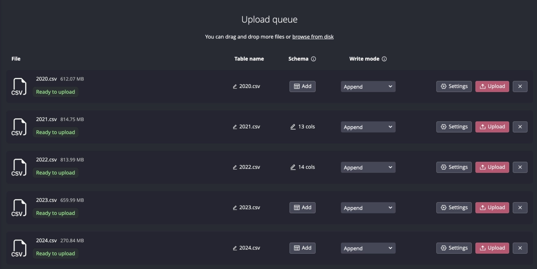
As is, the import leaves us with a bunch of tables named 2019.csv, 2020.csv,
etc. To use the data further, we need to combine all tables into one.
Additionally, the transaction date field called date_mutation has been
imported as a varchar. We want to first convert it to a timestamp type as
follows:
ALTER TABLE "2019.csv" ALTER COLUMN date_mutation TYPE timestamp;ALTER TABLE "2020.csv" ALTER COLUMN date_mutation TYPE timestamp;ALTER TABLE "2021.csv" ALTER COLUMN date_mutation TYPE timestamp;ALTER TABLE "2022.csv" ALTER COLUMN date_mutation TYPE timestamp;ALTER TABLE "2023.csv" ALTER COLUMN date_mutation TYPE timestamp;ALTER TABLE "2024.csv" ALTER COLUMN date_mutation TYPE timestamp;
We can then run a CREATE TABLE ... AS command to populate a new table which
will combine all of the above and be indexed by timestamp:
CREATE TABLE dvf AS(SELECT * FROM (SELECT * FROM "2019.csv"UNION ALLSELECT * FROM "2020.csv"UNION ALLSELECT * FROM "2021.csv"UNION ALLSELECT * FROM "2022.csv"UNION ALLSELECT * FROM "2023.csv"UNION ALLSELECT * FROM "2024.csv") order by date_mutation) timestamp(date_mutation)
While we're at it, we can set some varchar columns to symbol and add an
index. Both these operations will reduce the amount of disk space consumed by
the data, and accelerate queries based on these fields:
ALTER TABLE dvf ALTER COLUMN nature_mutation TYPE symbol;ALTER TABLE dvf ALTER COLUMN code_postal TYPE symbol;ALTER TABLE dvf ALTER COLUMN nom_commune TYPE symbol;ALTER TABLE dvf ALTER COLUMN nature_mutation ADD INDEX;ALTER TABLE dvf ALTER COLUMN code_postal ADD INDEX;ALTER TABLE dvf ALTER COLUMN nom_commune ADD INDEX;
Data sanitation
We can get a few ideas about the dataset with a few simple queries.
SELECT year(date_mutation), count() FROM dvf ORDER BY year ASC;
| year | count |
|---|---|
| 2019 | 1,967,866 |
| 2020 | 3,522,100 |
| 2021 | 4,672,561 |
| 2022 | 4,667,090 |
| 2023 | 3,799,407 |
| 2024 | 1,566,643 |
The years 2019 and 2024 are only partial so this dataset is about 3-5 million transactions per year, for a total of around 20 million transactions.
The field nature_mutation contains the type of property transfer.
SELECT DISTINCT nature_mutation FROM dvf
This returns the following values:
vente: saleechange: exchangeVente en l'etat futur d'achevement: properties sold off plansVente terrain a batir: sale of constructible landAdjudication: sold through auctionExpropriation: expropriated
For the subsequent analysis, we will focus on outright sales to make it easier to compare results. In a similar way, we will filter results on house and apartment sales only, and exclude industrial or commercial properties. Additionally, we can see many duplicates in the data, so we will sanitise it and remove them.
Most of these duplicates are block transactions with multiple properties. However, each subtransaction is reported with the full transaction amount rather than a portion.
So for example, for a sale of 10 apartments, we'll see 10 transactions for 1,000,000 EUR. But this amount is the total transaction amount. A more realistic representation would be, for example, 10 transactions for 100,000 EUR each.
Lastly, I'd like to get rid of certain fields and calculate other derived fields such as the price per square meter. Therefore, I'll create a copy of the dataset as follows which will achieve these objectives:
CREATE TABLE dvf_data as (WITH ids as (SELECT id_mutationFROM (SELECT id_mutation, count() FROM dvf)WHERE count = 1)SELECT DISTINCTids.id_mutation id, date_mutation dt, valeur_fonciere price, adresse_nom_voie street,code_departement department, type_local type,surface_reelle_bati surface, longitude, latitude, code_postal postcode,nom_commune city, cast(valeur_fonciere/surface_reelle_bati as int) price_sqmFROMdvf JOIN ids ON dvf.id_mutation = ids.id_mutationWHEREnature_mutation = 'Vente'AND (type_local = 'Maison' OR type_local = 'Appartement'))
This leaves us with 1.7 million transactions, which correspond to unique sales of houses and apartments. With this ready, we can start doing some analysis.
What's the industry trend?
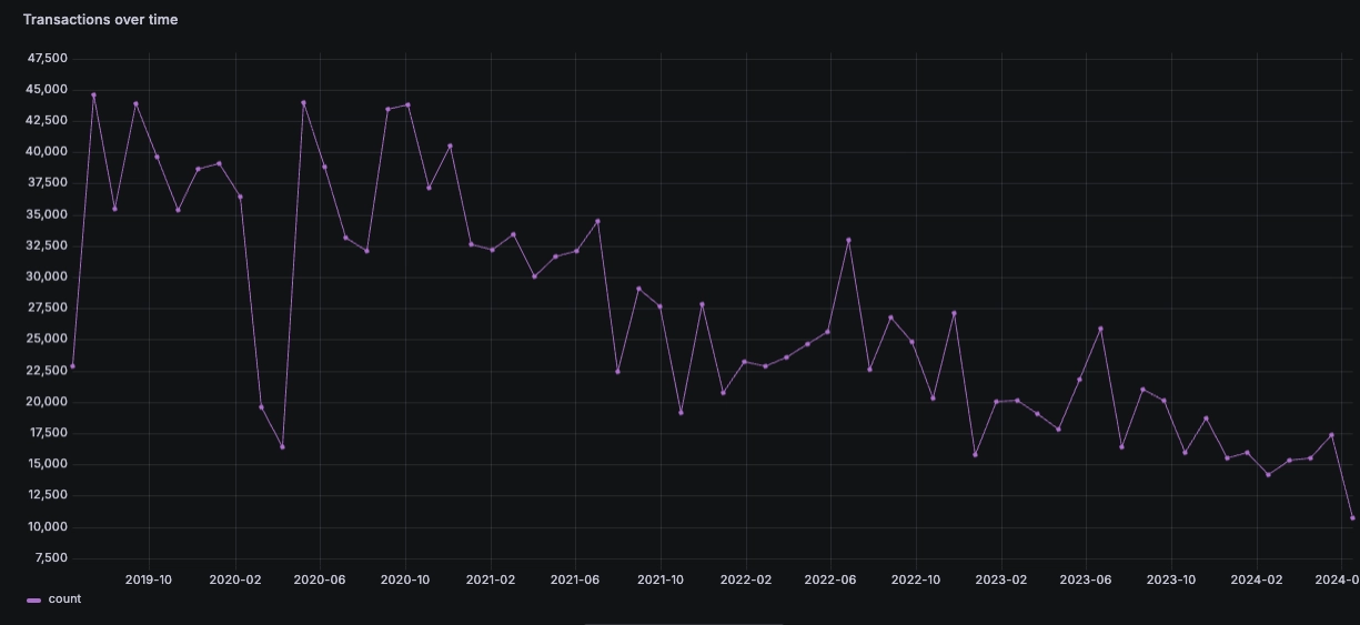
Since we have timestamped data, we can try to look at a few trends. The first instinctive items to look at would be the number of transactions and the total amount transacted:
SELECT dt, count() FROM dvf_data SAMPLE BY 30d
Let's roll this and some other queries into Grafana charts.
Assuming we sanitised the data correctly, the result suggests a structural decline in the number of transactions realised in France since 2019.
A similar query with SUM(..) .. SAMPLE BY shows a similar decline in the
amount transacted:
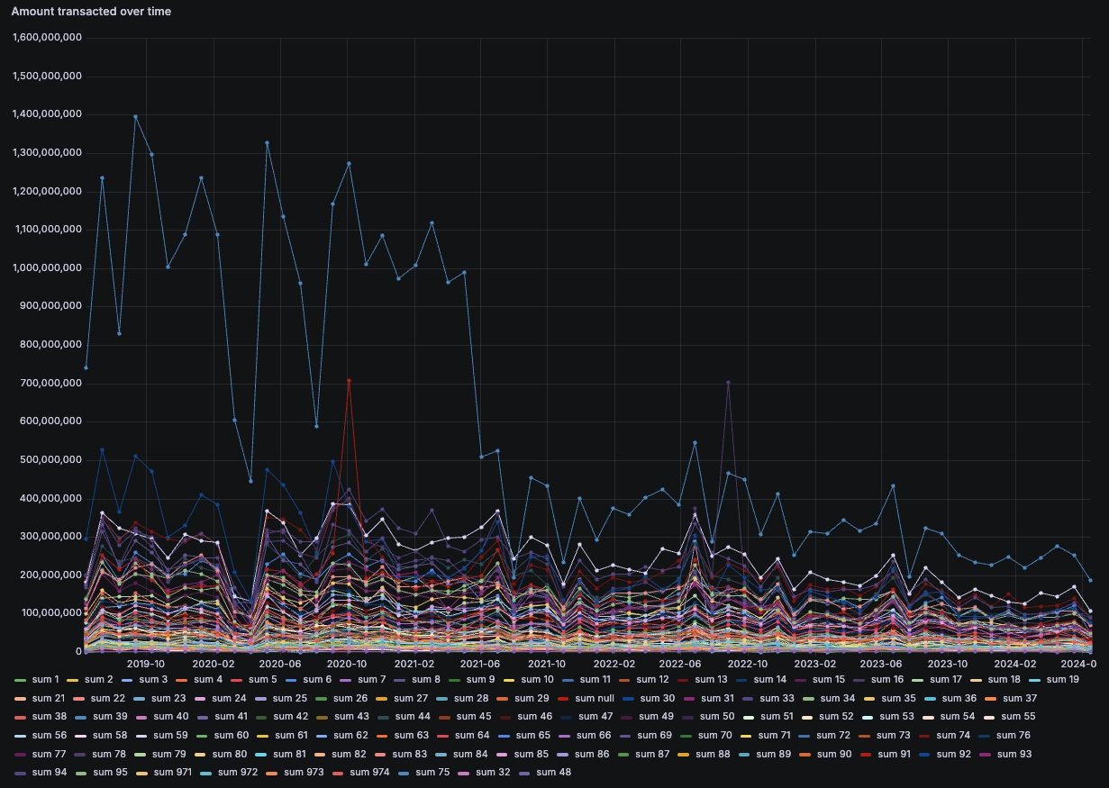
If we add granularity by department, then we can see the main culprit seems to
be Paris (Department code 75):
SELECT dt, department, sum(price) FROM dvf_data SAMPLE BY 30d
However, when excluding Paris, the total number of transactions is still in decline. While Paris saw a large decrease with COVID, it seems the decrease in transaction count and amount is generalised across regions:
# Transactions by regionSELECT dt, sum(price) all_regions FROM dvf_data SAMPLE BY 30d# Transactions excluding ParisSELECT dt, sum(price) excl_paris FROM dvf_data WHERE department != 75 SAMPLE BY 30d
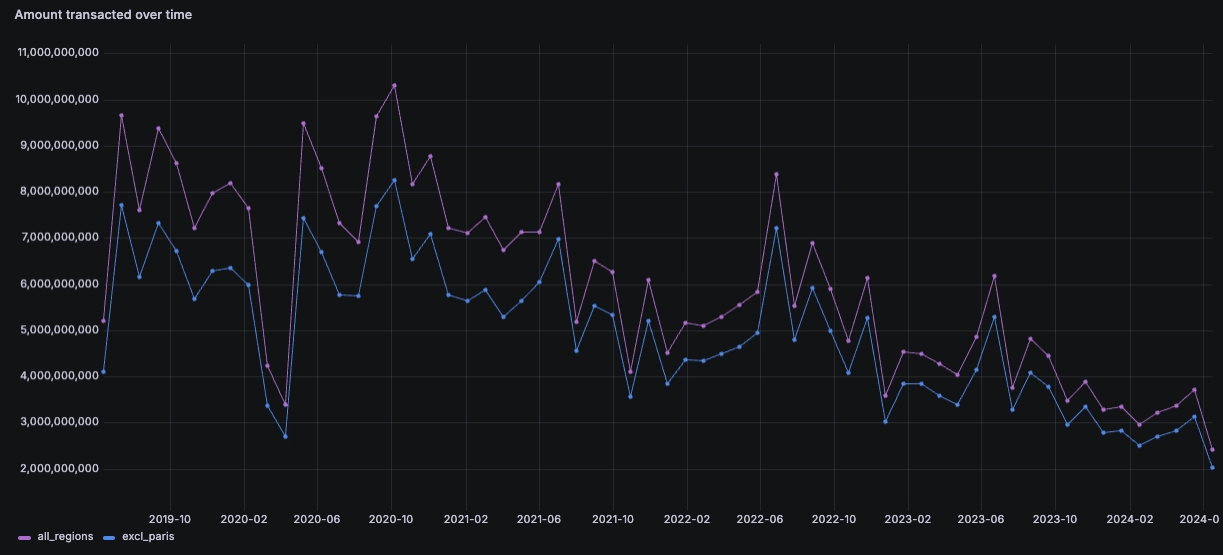
Since real-estate agents are paid via commissions proportional to the amount transacted, it seems logical that the revenue in this industry is likely in decline, alongside other related activities such as notary offices.
Prices always go up?
I don't know about your parents, but mine tell me I should buy now without thinking because real-estate prices always go up (allegedly). Let's see if we can corroborate this through data analysis.
First, let's compare the average transaction amount across all regions. We should note that this approach has severe limits. Within this calculation, we are comparing 1-bed flats and mansions without any adjustment. But it will give us a basic idea:
SELECT dt, avg(price) average_price FROM dvf_data SAMPLE BY 30d
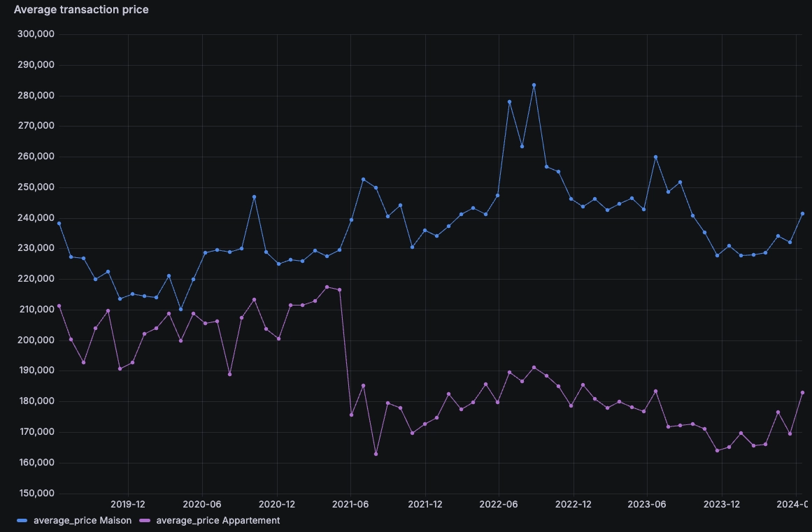
So the first thing I can say is that I'm glad I didn't buy in 2022! Prices don't always go up, and in this case, a tighter monetary policy and perhaps a cooldown following a potential real-estate bubble have taken prices down since their peak.
Exodus from the cities
What's most interesting is the gap change between houses and apartments. Naturally, houses transact at a premium over apartments. However, this premium increased sharply with COVID as the price of apartments fell. Looking only at house prices, it may seem like prices increased sharply until a peak in 2022, but this seems to have corrected since.
Now, these stats are at a national level. But if we correlate this with the amount of transactions in Paris and so on, it seems that this could be revealing.
Let's add some granularity and focus on Paris vs surrounding departments:
SELECT dt, department, avg(price) FROM dvf_dataWHERE price < 2000000 AND (department = 75 OR department = 77 OR department = 91 OR department = 92OR department = 93 OR department = 94 OR department = 95)SAMPLE BY 30d
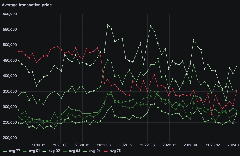
This one is quite interesting and telling about the exodus from Paris (75) to the periphery (77, 91, 92, etc.). Prices dropped sharply in paris in June 2021 while they increased in all the surrounding, less dense, areas.
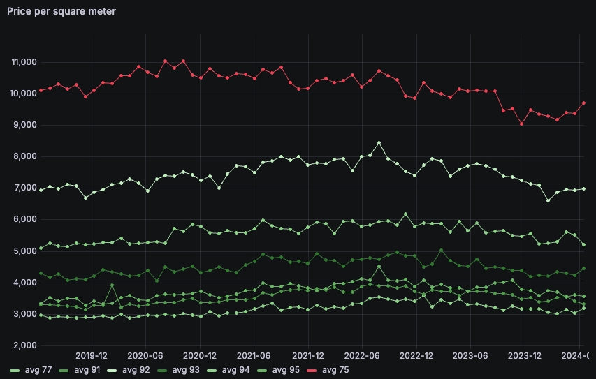
Perhaps one of the reasons is that you get more bang for your buck in the periphery. If we look at the prices divided by the surface, we end up with the price per square meter.
Paris remains an outlier with prices between 9-11k per meter while other regions are half or less. So for example, you can get 3x the space for the same money in the 77th department compared to Paris:
SELECT dt, department, avg(price_sqm) FROM dvf_dataWHERE price < 2000000 AND (department = 75 OR department = 77 OR department = 91 OR department = 92OR department = 93 OR department = 94 OR department = 95)SAMPLE BY 30d
Playing with Grafana maps
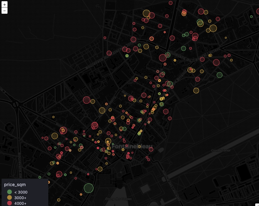
One nice thing about the DVF dataset is that it includes the unique parcel identifier. An even nicer thing about it is that some folks enriched the dataset by cross-referencing it with cadastral data to include the coordinates of each parcel. When we overlay both together, we end up with geolocated transactional data which we can display in a Grafana Geomap.
In this example, we can zoom on a particular city by filtering on the postcode field. From there, we can overlay coordinates, surface (circle size), and price per square meter (circle color).
To create this map in Grafana, we modified the options to set the color scheme to From threshold, and also mapped the circle size to the surface field of my query:
SELECT latitude, longitude, price_sqm, surfaceFROM dvf_dataWHERE postcode = 77300AND price_sqm > 0 AND price_sqm < 5000
We can have more fun with maps of course, and use them to display heatmaps of price per square meter for example:
# Query 1: high prices (red)SELECT latitude, longitude, price_sqm from dvf_dataWHERE price_sqm > 10000 and latitude > 41# Query 2 : low prices (green)SELECT latitude, longitude, price_sqm from dvf_dataWHERE price_sqm < 2000 and latitude > 41LIMIT 10000
If you're wondering why we're filtering on latitude, this is because the DVF dataset includes overseas territories such as Guyane, Guadeloupe, Reunion Island and others.
By filtering on latitude, we focus the map on metropolitan France:
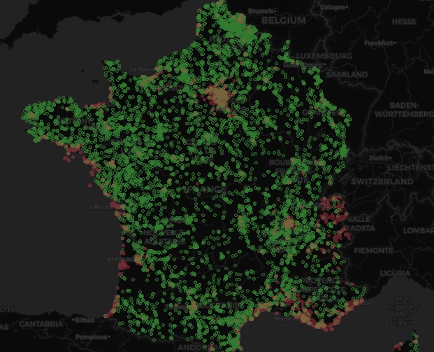
In this instance, we see two layers. One with high prices per square meter (> 10,000 EUR), and another with low prices (< 3,000 EUR). Interestingly and intuitively, we can see clusters of high prices around Paris, on the Atlantic coast, on the mediterranean coast, and near the border with Switzerland.
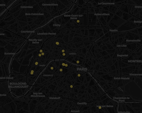
We can push the maps a bit more into showing us high ticker transactions, such as those above 10 million EUR:
SELECT latitude, longitude, price_sqm FROM dvf_dataWHERE price > 10000000 AND latitude > 41
In this map we can see some of the transactions above 10,000,000 EUR in the capital. Some properties reach 100k per square meter!
Some perspective
There's so much we could go and explore with this dataset. It tells so many stories. It tells us about COVID, interest rates tightening, exodus from the capital to the suburbs, and it covers both transactions from billionaires and ordinary people.
With so many possibilities, it's hard to take this post to a conclusion. But I think this example perfectly illustrates the wealth gap which this dataset makes so visible:
SELECT city, price, surface, price_sqm, streetFROM dvf_data WHERE price > 0 AND price_sqm < 100000ORDER BY price DESC LIMIT 100
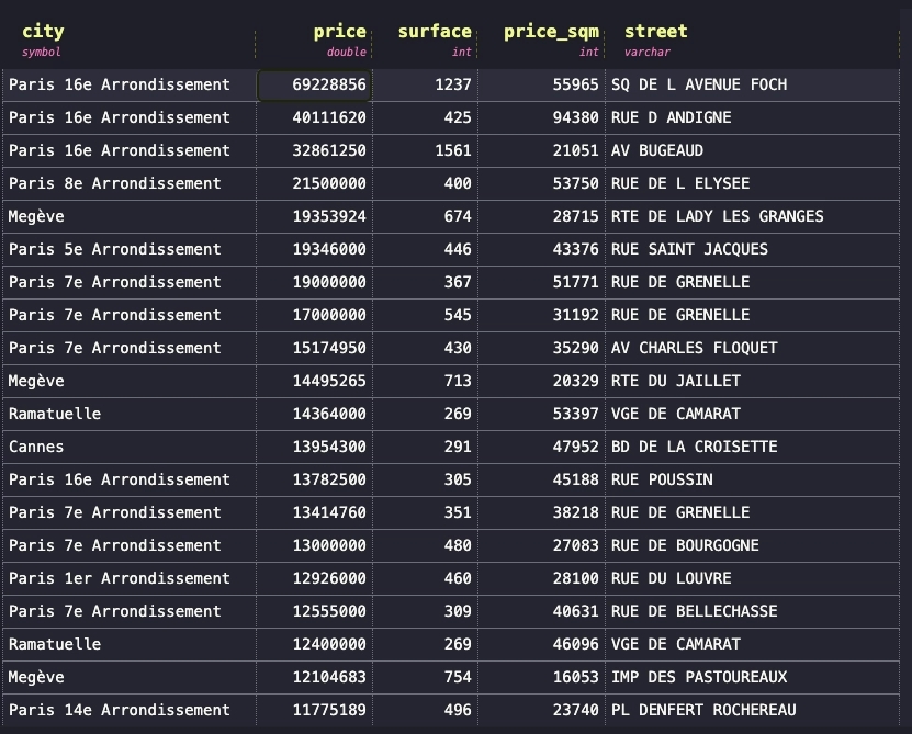
These are the most astronomical prices. Mostly in Paris, Megeve (a fancy ski resort), and Cannes (heard of the cinema festival?). One of these transactions reached a price of 94,380 EUR per square meter.
That's shocking! What else could you buy with this?
SELECT city, price, surface, price_sqm, streetFROM dvf_data WHERE price > 0 AND price < 94380'
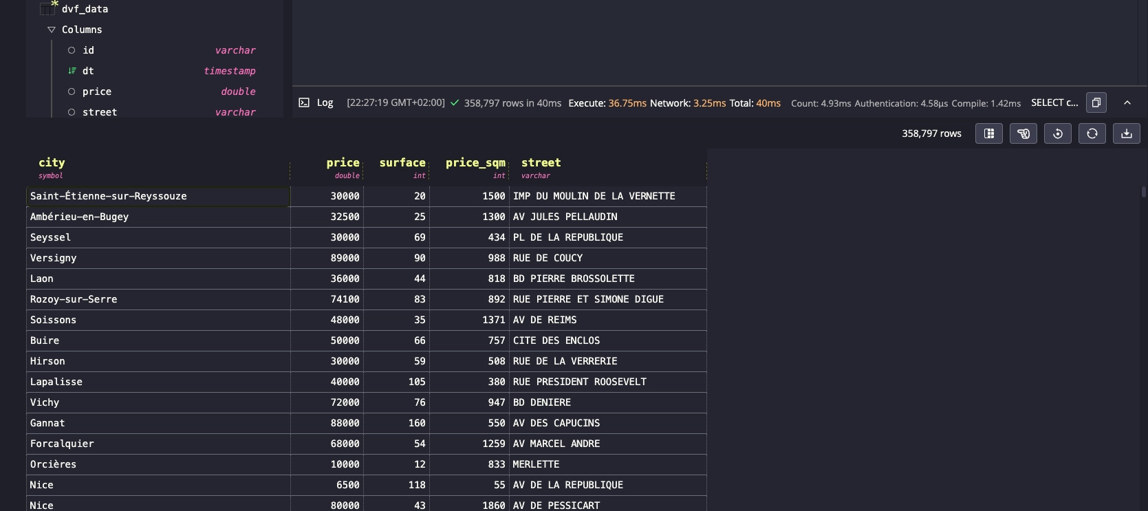
So for the price of 1 square meter Rue D'andigne in Paris (94380 EUR), you could buy any of 358,000 properties. Put differently, with the price spent to purchase single flat, one could have bought outright houses and apartments for 425 families.
Summary
This dive into the French real estate market, using QuestDB and Grafana, uncovers trends in property transactions, price fluctuations, and regional differences since COVID. We revealed insights into the impact of rising interest rates, the shift from urban to suburban areas, and the overall health of the industry. With Grafana visualizations and QuestDB queries, the DVF dataset tells us some fascinating stories about real estate in France.
If you'd like to chat or ask questions, please drop by our Community Forum or our public Slack.
Interested in more Grafana tutorials?
Check these out:
- Fluid real-time dashboards with QuestDB and Grafana
- Build your own resource monitor
- Tracking sea faring ships with AIS data and Grafana
- Visualizing real-time NYC cab data and geodata
- Analyzing the beautiful charts and history behind ECB FX rates
- Increase Grafana refresh rate frequency
- Or check out our Grafana blog tag