Visualizing IoT Data with MQTT, QuestDB, and Grafana

Monitoring Time-series IoT Device Data​

Time-series data is crucial for IoT device monitoring and data visualization in industries such as agriculture, renewable energy, and meteorology. It enables trend analysis, anomaly detection, and predictive analytics, empowering businesses to optimize performance and make data-driven decisions. Thanks to technological advancements and the accessibility of open-source tools, gathering and analyzing data from IoT devices has become easier than ever before.

In this tutorial, we will guide you through the process of setting up a monitoring system for IoT device data. We will use historical electricity consumption data from some European countries, captured at a 15-minute resolution. The data is sent to an MQTT-compatible message broker called Mosquitto, and then channeled to QuestDB through Telegraf, a highly efficient data collector. To visualize the results, we will connect Grafana to QuestDB using its Postgres interface.

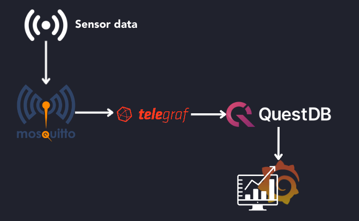
Since we don't have our own sensors to collect the data and send it directly to the broker, we will create the scenario by having a script that gathers the electricity consumption data from Open Power System Data and sends it to Mosquitto.

Prerequisites​

Before delving into the system setup, please make sure that you have installed the following:

• Docker
• The latest Go version

Setting up the prerequisites​

To get started, clone the prepared GitHub repository:

git clone https://github.com/questdb/questdb-mock-power-sensor mock-sensor

This repository contains all the configuration files and mock sensor scripts we will need during the tutorial.

Furthermore, we are going to need a new Docker network named "tutorial" to enable communication between containers without installing additional software on the host system. To create the new network, execute the following command:

docker network create tutorial

Setting up an MQTT broker​

To enable communication between IoT devices and the monitoring system, we need a message broker such as Eclipse Mosquitto, which implements the lightweight MQTT protocol. By using Eclipse Mosquitto, we establish a reliable and efficient communication channel for IoT devices.

To run Eclipse Mosquitto, we are going to use Docker. The default configuration for Mosquitto does not allow unauthenticated clients. However, no default credentials are set. To fix this, let's use the conf/mosquitto/mosquitto.conf to override the default settings:

allow_anonymous true
listener 1883 0.0.0.0

To start the Eclipse Mosquitto broker using Docker, you can execute the following command from the repository root:

docker run --rm -dit -p 1883:1883 -p 9001:9001 \
 -v "$(pwd)"/conf/mosquitto/mosquitto.conf:/mosquitto/config/mosquitto.conf \
 --network=tutorial --name=mosquitto eclipse-mosquitto

By running this command, the Eclipse Mosquitto broker will start within a Docker container, configured with the settings from the mosquitto.conf file. The specified ports will be exposed to enable MQTT communication and the container will be connected to the tutorial Docker network, allowing it to communicate with other containers in the network.

Tunneling data into Mosquitto​

Now that the message broker is running, in a new terminal window, navigate to the repository root and start the script that will populate the data for us:

cd script
go get
go run ./main.go

Great! The script will continue running in the background until it is manually stopped or until it runs out of data to publish. Since we are using a historical dataset, the script will override the original timestamps with the current time when sending the records to the MQTT broker.

With a 1-second delay between records, the script will consistently publish data to the broker, ensuring a steady flow of simulated sensor data for your tutorial. This allows you to progress with the rest of the tutorial without worrying about starting or stopping the script manually.

Setting up QuestDB​

To ensure that all incoming IoT data flowing through Mosquitto is stored in QuestDB by the end of this tutorial, let's start QuestDB in the background. This will allow us to connect to it later using Telegraf.

Execute the following Docker command to start QuestDB:

docker run --rm -dit -p 8812:8812 -p 9000:9000 \
    -p 9009:9009 -e QDB_PG_READONLY_USER_ENABLED=true \
    --network=tutorial --name=questdb questdb/questdb

Once the command is executed, QuestDB will start running in the background. To validate that QuestDB is up and running, you can visit http://localhost:9000 in your web browser.

By accessing the provided URL, you should be able to access the QuestDB web interface, indicating that QuestDB has been successfully started.

Connecting the dots and adding Telegraf​

In this setup, Telegraf will play a key role in transferring data between Mosquitto and QuestDB. To enable this seamless data transfer, we will utilize QuestDB's ILP (Influx Line Protocol) interface, as ILP is capable of handling large volumes of data efficiently sent from Telegraf.

To configure Telegraf, we are using the conf/telegraf/telegraf.conf file, which has the following content:

# Configuration for Telegraf agent
[agent]
  ## Default data collection interval for all inputs
  interval = "1s"

[[inputs.mqtt_consumer]]
  servers = ["tcp://mosquitto:1883"]
  topics = ["sensor"]
  data_format = "influx"
  client_id = "telegraf"
  data_type = "string"

# Write results to QuestDB
[[outputs.socket_writer]]
  # Write metrics to a local QuestDB instance over TCP
  address = "tcp://questdb:9009"

Let’s start the Telegraf container by executing:

docker run --rm -it \
    -v "$(pwd)"/conf/telegraf/telegraf.conf:/etc/telegraf/telegraf.conf \
    --network=tutorial --name=telegraf telegraf

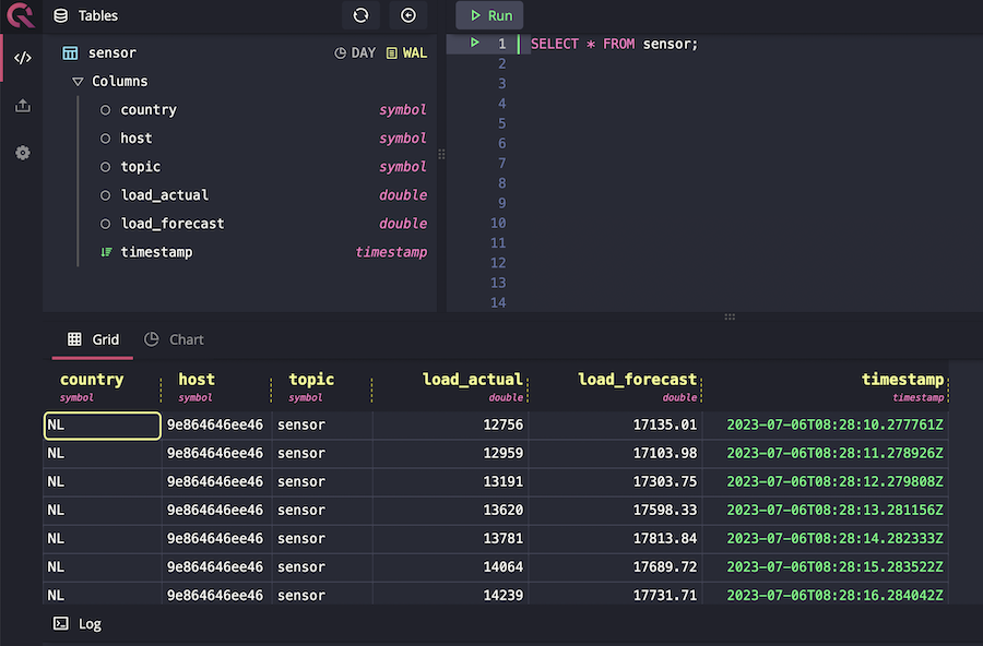
Once Telegraf is up and running, the sensor data is automatically tunneled into QuestDB, and a new table called "sensor" is created to store the incoming data. To verify that the data is successfully flowing into QuestDB, you can execute the following query on the QuestDB console, accessible at http://localhost:9000:

SELECT * FROM sensor;

In the next steps of the tutorial, we will set up Grafana, which is a powerful data visualization and monitoring tool. We will connect Grafana to QuestDB and create compelling visualizations based on the received sensor data.

Visualizing the dataset with Grafana​

To proceed with creating a Grafana container and connecting it to QuestDB, execute the following command:

docker run --rm -dit -p 3000:3000 \
    --network=tutorial --name=grafana grafana/grafana

This command will start a Grafana container within the same tutorial network. To access the Grafana login page, navigate to http://localhost:3000 in your web browser. You will be prompted to log in using the default credentials:

• Username: admin
• Password: admin

To connect Grafana with QuestDB and establish a data source, follow these steps:

1. Open your web browser and go to http://localhost:3000/datasources/new.
2. On the "New data source" page, select "PostgreSQL" as the data source type from the list of available options.

Fill in the form with the following details:

• Name: QuestDB
• Host: questdb:8812
• Database: qdb
• User: user
• Password: quest
• TLS/SSL mode: disable

Once you have filled in the form with the correct information, click on the "Save & Test" button at the bottom of the page. Grafana will attempt to connect to QuestDB using the provided credentials and verify the connection. If everything is set up correctly, you should see a success message indicating that the data source was added successfully.

Now that Grafana is successfully connected to QuestDB, you can begin creating insightful dashboards to visualize the electricity consumption data. Follow these steps to create a new dashboard:

1. In your browser and navigate to the new dashboard at http://localhost:3000/dashboard/new?orgId=1page.
2. Once you're on the new dashboard page, click on the "Add visualization" button.

On the popup panel, select “QuestDB” data source.

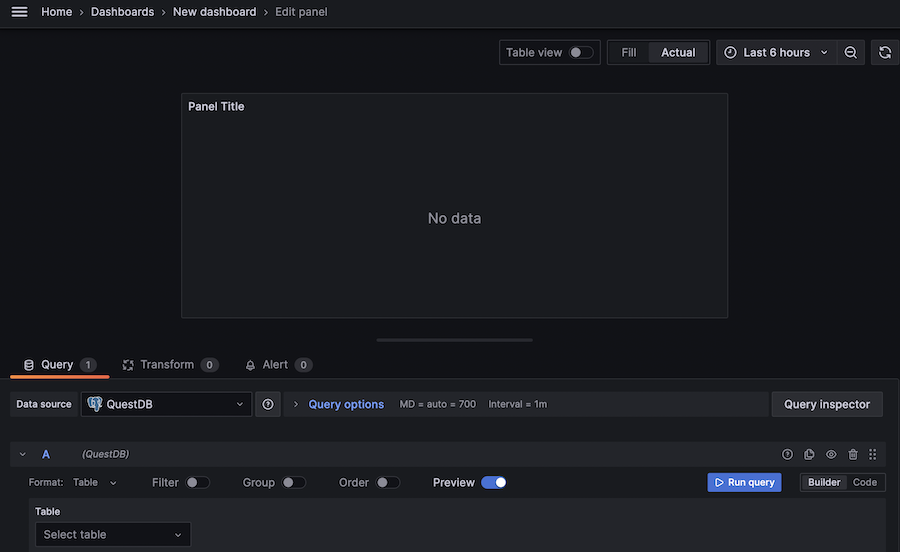
Now you're ready to start building your dashboard and visualizing the electricity consumption data from QuestDB. Grafana provides a wide range of visualization options, including graphs, charts, tables, and more. You can customize the panel settings, apply different visualization types, and configure data queries to create meaningful visual representations of the data.

To visualize the electricity consumption data from QuestDB, we will use the "Time series" chart type, which is the default selected chart based on our data. The "Time series" chart is ideal for displaying data over time and is well-suited for analyzing trends and patterns.

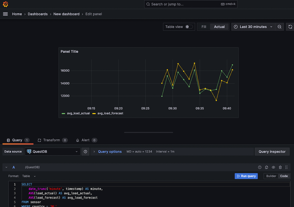
In the query builder panel, switch to “Code” and paste the following SQL query:

SELECT
    date_trunc('minute', timestamp) AS minute,
    AVG(load_actual) AS avg_load_actual,
    AVG(load_forecast) AS avg_load_forecast
FROM sensor
WHERE country = 'NL'
GROUP BY minute
ORDER BY minute ASC

By executing this query, we will obtain a result set that provides minutely aggregated data, showing the average, actual, and forecasted energy load for each minute. Feel free to adjust the sampling or grouping interval if you wish. If you followed this tutorial successfully, you should see similar results.

To make the changes persistent while the container is running, rename the title of the graph on the right-hand side properties pane, and save it by clicking on the “Apply” button in the top right corner.

The time series chart we have created, with the average actual and forecasted energy consumption, provides valuable insights into the accuracy of the forecasting logic. By analyzing this chart, we can easily identify any discrepancies between the actual and forecasted values, helping you pinpoint areas where improvements can be made.

Cleaning up resources​

Upon finishing the tutorial, you may want to clean up any dangling resources, such as the tutorial network we created. Removing a network requires the removal of existing resources attached to that first. To remove the containers, the network, and the images used during this tutorial, run the following commands:

docker ps -qa --filter="network=tutorial" | xargs -n1 docker kill
docker network rm tutorial
docker rmi telegraf eclipse-mosquitto grafana/grafana questdb/questdb

Summary​

In this tutorial, we explored the setup and configuration of a monitoring system for IoT device data using MQTT, Telegraf, QuestDB, and Grafana. Through a series of steps, we established communication between IoT devices and the monitoring system using Eclipse-Mosquitto as the MQTT broker.

We simulated data collection using a script that gathered electricity consumption from Open Power System Data and sent it to the MQTT broker. We stored this data in QuestDB and visualized it using Grafana. By connecting Grafana to QuestDB, we created informative dashboards to gain insights.

The tutorial showcased the power of time-series data and its visualization, enabling us to compare actual and forecasted energy consumption.