Weather data visualization and forecasting with QuestDB, Kafka and Grafana

Weather stations, satellites, and sensor arrays generate a ton of weather-related events every millisecond. When captured, this data can go on to become valuable for various applications such as agriculture, transportation, energy, and disaster management. For this, a specialized time-series database like QuestDB can help store and efficiently process large volumes of data.

In this tutorial, we will stream and visualize large volumes of data into QuestDB. To do so, we'll use Kafka, a distributed streaming platform that can handle high-volume data streams. Then, we will apply Grafana, a powerful open-source data visualization tool, to create a cool dashboard for weather forecasting.

Prerequisites​

To follow along with this tutorial, you will require:

• A Docker environment set up on your machine
• Docker images for Grafana, Kafka, and QuestDB
• Node.js and npm
• Basic knowledge of Node.js, Express.js, Kafka, and Grafana

Node.js application setup​

To start, we'll create a pair of microservices. One service will be the Kafka stream provider, and the other service will consume these data streams for storage in QuestDB.

First, create a new directory for your project and navigate into it:

mkdir weather-data-visualization
cd weather-data-visualization

Then, create a new Node.js project using the npm command:

npm init -y

Next, install the following dependencies:

npm install @questdb/nodejs-client dotenv express kafkajs node-cron node-fetch

• @questdb/nodejs-client: The official QuestDB Node client library
• dotenv: Zero-dependency module that loads environment variables from an env file into process.env
• express: Minimal Node web application framework
• kafkajs: Kafka client for Node
• node-cron: Simple and lightweight cron-like job scheduler for Node
• node-fetch: A lightweight module which brings the window.fetch API to Node

The next step is to create a new file named .env and add the following environment variables:

PORTA=3001
PORTB=3002
WEATHER_API_KEY=<your-openweather-api-key>

For guidance towards safe storage of environment variables, checkout this guide.

Kafka streaming service​

Now, with node setup, let's create the services for the application.

We need two services:

1. one to stream the weather data from the OpenWeatherMap API
2. another to consume the data streams and store them in QuestDB

To this end, we will create two new directories named app-producer and app-consumer in the root directory and add a new file called index.js to each.

For the index.js file in the app-producer service, we'll add the following code:

import express from "express"
import dotenv from "dotenv"
import { Kafka } from "kafkajs"
import cron from "node-cron"
import fetch from "node-fetch"

dotenv.config()

const API_KEY = process.env.WEATHER_API_KEY

const cities = [
  { name: "New York", lat: 40.7128, lon: -74.006 },
  { name: "São Paulo", lat: -23.5505, lon: -46.6333 },
  { name: "London", lat: 51.5074, lon: -0.1278 },
  { name: "Cairo", lat: 30.0444, lon: 31.2357 },
  { name: "Sydney", lat: -33.8688, lon: 151.2093 },
  { name: "Tokyo", lat: 35.6895, lon: 139.6917 },
  { name: "Moscow", lat: 55.7558, lon: 37.6173 },
  { name: "Mumbai", lat: 19.076, lon: 72.8777 },
  { name: "Buenos Aires", lat: -34.6037, lon: -58.3816 },
  { name: "Cape Town", lat: -33.9249, lon: 18.4241 },
]

const app = express()
app.use(express.json())

const kafka = new Kafka({
  clientId: "weather-producer",
  brokers: ["kafka:29092"],
})

const producer = kafka.producer()

// Add health check route
app.get("/health", (req, res) => {
  res.status(200).json({ status: "OK", message: "Producer service is healthy" })
})

// Your logic for fetching, processing, and sending weather data to Kafka will go here

app.listen(process.env.PORTA, () => {
  console.log("Weather Producer running on port", process.env.PORTA)
})

In this file, we create an Express app, connect to the Kafka network, and initialize a Kafka producer. We also add a health check route to the app so that we can confirm it's running well. The Express app is then set to listen to the port specified in the .env file.

Fetch weather data​

After setting up the Express app and health check, we need code to fetch the weather data. The first addition is the function that fetches the weather data. To the index.js file in the app-consumer service after the health check route, we'll add the following code:

async function fetchWeatherData(lat, lon) {
  const currentTime = Math.floor(Date.now() / 1000)
  try {
    const response = await fetch(
      `https://api.openweathermap.org/data/3.0/onecall/timemachine?lat=${lat}&lon=${lon}&dt=${currentTime}&units=metric&appid=${API_KEY}`,
    )
    if (!response.ok) {
      throw new Error(`HTTP error! status: ${response.status}`)
    }
    return await response.json()
  } catch (error) {
    console.error("Error fetching weather data:", error)
    return null
  }
}

The fetchWeatherData() function fetches the weather data from the OpenWeatherMap API. It's free to use, and very useful for demo purposes.

Process weather data​

Now it is time to process the weather data. An additional function will check if the fetchWeatherData() function returns data. If there is none, it returns an empty array. When there is data, it returns an object that matches the QuestDB schema.

Again in the index.js file in the app-producer service, below the fetchWeatherData() function, we'll add the following code:

function processWeatherData(data, city) {
  if (!data || !data.data || data.data.length === 0) {
    console.error("Invalid weather data received")
    return []
  }

  const current = data.data[0]
  // Convert Unix timestamps to microseconds
  const toDBTime = (unixTimestamp) => {
    const toISO = new Date(unixTimestamp * 1000)
    const dateObj = new Date(toISO)
    const toMicroseconds = BigInt(dateObj.getTime()) * 1000n
    console.log(toMicroseconds)

    return toMicroseconds
  }

  return {
    city: city.name,
    timezone: data.timezone,
    timestamp: toDBTime(current.dt),
    temperature: current.temp,
    sunrise: toDBTime(current.sunrise),
    sunset: toDBTime(current.sunset),
    feels_like: current.feels_like,
    pressure: current.pressure,
    humidity: current.humidity,
    clouds: current.clouds,
    weather_main: current.weather[0].main,
    weather_description: current.weather[0].description,
    weather_icon: current.weather[0].icon,
  }
}

This processWeatherData() function processes the weather data and returns a list of objects to stream to Kafka and save to the database.

Send data to Kafka​

Time to involve Kafka. For this, we'll create yet another function to send the processed data to the Kafka topic. Our new function will take an array of data, check for fields in each object that is of type BigInt, then convert it to string so that we can stream it via Kafka.

We do the conversion due to Kafka's preference for serialized messages. JSON is the most common vehicle for this. JSON does not natively support BigInt. So, the conversion allows safe streaming to Kafka without any serialization errors.

In the index.js file in the app-producer service, below the processWeatherData() function, add the following code:

async function sendToKafka(data) {
  try {
    await producer.connect()
    const messages = data.map((item) => ({
      value: JSON.stringify(item, (key, value) =>
        typeof value === "bigint" ? value.toString() : value,
      ),
    }))
    await producer.send({
      topic: "weather-data",
      messages,
    })
  } catch (error) {
    console.error("Error sending data to Kafka:", error)
  } finally {
    await producer.disconnect()
  }
}

With this, the sendToKafka() function sends the processed data to the Kafka topic.

Schedule task​

Finally, we will create one more function to schedule the task to run every 15 minutes. It will fetch fresh weather data and send it to the Kafka topic:

async function generateWeatherData() {
  const weatherDataPromises = cities.map((city) =>
    fetchWeatherData(city.lat, city.lon),
  )
  const weatherDataResults = await Promise.all(weatherDataPromises)

  const processedData = weatherDataResults
    .map((data, index) => processWeatherData(data, cities[index]))
    .filter((data) => data !== null)

  if (processedData.length > 0) {
    await sendToKafka(processedData)
  }
  return processedData
}

// Initial run
generateWeatherData().then((data) => {
  if (data) {
    console.log("Initial weather data sent to Kafka:", data)
  }
})

// Schedule the task to run every 15 minutes
cron.schedule("*/15 * * * *", async () => {
  const weatherData = await generateWeatherData()
  if (weatherData) {
    console.log("Weather data sent to Kafka:", weatherData)
  }
})

The generateWeatherData() function triggers the initial call for the above function in the order outlined above – fetch weather information, process it, and send it to the Kafka topic. It then schedules the task to run every 15 minutes.

Things to note:

• The OpenWeatherAPI call is to get the current weather report of the cities defined above. The cron package schedules the task to run every 15 minutes. You can add as many cities as you want. Also, note that the free tier of this API is limited to 60 calls per minute.
• The toDBTime() function formats the Unix time to bigint. The QuestDB Node.js client only supports the epoch(microseconds) or bigint data type for timestamps.

Saving to QuestDB​

It's QuestDB's turn.

In this section, we connect QuestDB to the Kafka producer and consume the weather data from the Kafka weather topic in the app-consumer service app. We also add another health check route to the app.

In the index.js file in the app-consumer service, we'll add the following starter code:

import express from "express"
import dotenv from "dotenv"
import { Kafka } from "kafkajs"
import { Sender } from "@questdb/nodejs-client"

dotenv.config()

const app = express()
app.use(express.json())

const kafka = new Kafka({
  clientId: "weather-consumer",
  brokers: ["kafka:29092"],
})

const consumer = kafka.consumer({
  groupId: "weather-group",
  retry: {
    retries: 8, // Increase the number of retries
  },
  requestTimeout: 60000, // Increase the request timeout
})

// Add health check route
app.get("/health", (req, res) => {
  res.status(200).json({ status: "OK", message: "Consumer service is healthy" })
})

// The logic for starting the consumer and processing the data to QuestDB will go here
//...
//...

app.listen(process.env.PORTB, () => {
  console.log("Weather Consumer running on port", process.env.PORTB)
})

Ingesting into QuestDB​

A new function will save data to QuestDB. To do so, We initialize a sender with QuestDB configuration details, then map the data from the producer service to our preferred schema. The sender is then flushed, and the connection is closed after saving the data:

async function saveToQuestDB(data) {
  const sender = Sender.fromConfig(
    "http::addr=questdb:9000;username=admin;password=quest;",
  )
  try {
    await sender
      .table("weather_data")
      .symbol("city", data.city)
      .symbol("timezone", data.timezone)
      .timestampColumn("timestamp", parseInt(data.timestamp))
      .floatColumn("temperature", data.temperature)
      .timestampColumn("sunrise", parseInt(data.sunrise))
      .timestampColumn("sunset", parseInt(data.sunset))
      .floatColumn("feels_like", data.feels_like)
      .floatColumn("pressure", data.pressure)
      .floatColumn("humidity", data.humidity)
      .stringColumn("weather_main", data.weather_main)
      .stringColumn("weather_desc", data.weather_description)
      .stringColumn("weather_icon", data.weather_icon)
      .at(Date.now(), "ms")
    console.log("Data saved to QuestDB")
  } catch (error) {
    console.error("Error saving data to QuestDB:", error)
  } finally {
    await sender.flush()
    await sender.close()
  }
}

The saveToDB() function defines the table and its schema. Note the fields we've deemed relevant and the types we've specified that make up our schema.

It's important to note here that the QuestDB clients leverage the InfluxDB Line Protocol (ILP) over HTTP. With ILP over HTTP, table creates are handled automatically. Once QuestDB receives this payload, the table is created as needed. That means no additional upfront work is required.

The data is sent, tables are created, and it's now within QuestDB.

Starting the consumer​

Now we need some logic to subscribe to the Kafka topic from the producer service. We also need to process stringified Kafka messages to JSON, and start the consumer:

async function processMessage(message) {
  const data = JSON.parse(message.value.toString())
  console.log("Received weather data:", data)
  await saveToQuestDB(data)
}

async function startConsumer() {
  await consumer.connect()
  await consumer.subscribe({ topic: "weather-data", fromBeginning: true })

  await consumer.run({
    eachMessage: async ({ message }) => {
      await processMessage(message)
    },
  })
}

process.on("SIGINT", async () => {
  console.log("Shutting down gracefully...")
  await consumer.disconnect()
  process.exit(0)
})

startConsumer().catch(console.error)

The processMessage() function processes and sends data to QuestDB. The startConsumer() function starts the consumer, subscribes to the topic from the provider, and utilizes the processMessage() function to process each stream of data.

In cases where the app is terminated, the process.on() function handles the graceful shutdown of the consumer.

Things to note:

• The sender configuration uses questdb:9000 instead of localhost:9000 because the QuestDB server runs inside a Docker container, and the hostname is questdb. Use localhost or whatever you set as hostname in your docker-compose.yml file.
• The timestampColumn data uses parseInt method to format the JSON data from the produce to integer since it only accepts unix time or bigint.

Dockerizing the app​

We have successfully built a service to get weather data from the OpenWeatherMap API, and then stream it to the Kafka broker. We also have another service to then consume and stream that data to QuestDB. Now let's dockerize these services.

In addition to the two services, we'll include a Grafana docker image, Kafka docker image, and our QuestDB docker image. This will enable our applications to interact with and between these applications. To that end, we will create a Dockerfile for each service.

The Dockerfile for the producer service will look like this:

FROM node:16.9.0-alpine
WORKDIR /app
COPY package.json app-producer/index.js /app/
RUN npm install
RUN npm i -g nodemon
CMD [ "nodemon", "index.js" ]

The Dockerfile for the consumer service will look like this:

FROM node:16.9.0-alpine
WORKDIR /app
COPY package.json app-consumer/index.js /app/
RUN npm install
RUN npm i -g nodemon
CMD [ "nodemon", "index.js" ]

These Dockerfiles are straightforward. We use the Node.js Alpine image and copy the package.json file from the root folder and the index.js file from the respective services to the image. We also install the dependencies and run the service using nodemon.

Next, we create a docker-compose.yml file in the root folder. This file will define the services and the networks to which they will connect:

services:
  app1:
    container_name: app-producer
    build:
      context: ./
      dockerfile: ./app-producer/Dockerfile
    ports:
      - "8080:3001"
    env_file:
      - ./.env
    depends_on:
      - kafka

  app2:
    container_name: app-consumer
    build:
      context: ./
      dockerfile: ./app-consumer/Dockerfile
    ports:
      - "8081:3002"
    env_file:
      - ./.env
    depends_on:
      - kafka

  questdb:
    image: questdb/questdb:8.1.0
    container_name: questdb
    ports:
      - "9000:9000"
    environment:
      - QDB_PG_READONLY_USER_ENABLED=true

  grafana:
    image: grafana/grafana-oss:11.1.3
    container_name: grafana
    ports:
      - "3000:3000"
    depends_on:
      - questdb

  zookeeper:
    image: confluentinc/cp-zookeeper:7.3.0
    container_name: zookeeper
    ports:
      - "2181:2181"
    environment:
      ZOOKEEPER_CLIENT_PORT: 2181
      ZOOKEEPER_TICK_TIME: 2000

  kafka:
    image: confluentinc/cp-kafka:7.3.0
    container_name: kafka
    ports:
      - "9092:9092"
    environment:
      KAFKA_BROKER_ID: 1
      KAFKA_ZOOKEEPER_CONNECT: zookeeper:2181
      KAFKA_ADVERTISED_LISTENERS: PLAINTEXT://kafka:29092,PLAINTEXT_HOST://localhost:9092
      KAFKA_LISTENER_SECURITY_PROTOCOL_MAP: PLAINTEXT:PLAINTEXT,PLAINTEXT_HOST:PLAINTEXT
      KAFKA_INTER_BROKER_LISTENER_NAME: PLAINTEXT
      KAFKA_OFFSETS_TOPIC_REPLICATION_FACTOR: 1
    depends_on:
      - zookeeper

networks:
  default:
    name: weather-data-visualization-network

The docker-compose.yml file defines the following services:

• app1 - Producer service that references the Dockerfile in the app-producer folder and the root folder as context. The service listens to port 8080 and exposes it to the host machine. The service also depends on the kafka service
• app2 - Consumer service also references the Dockerfile in the app-consumer folder and the root folder as context. The service listens to port 8081 and exposes it to the host machine. It also depends on the kafka service
• questdb - QuestDB service
• grafana - Grafana service
• zookeeper - The Zookeeper service, which the Kafka service uses to manage topics and partitions
• kafka - Kafka service, which we connect to the weather-data-visualization-network network

We've also defined the environmental variables for each service. The env_file property defines the environment variables from the .env file.

With this setup, we're ready to build the images and run the services.

Building and running the app​

The app is ready to run on docker containers.

Build the images and run the services using the following docker-compose commands:

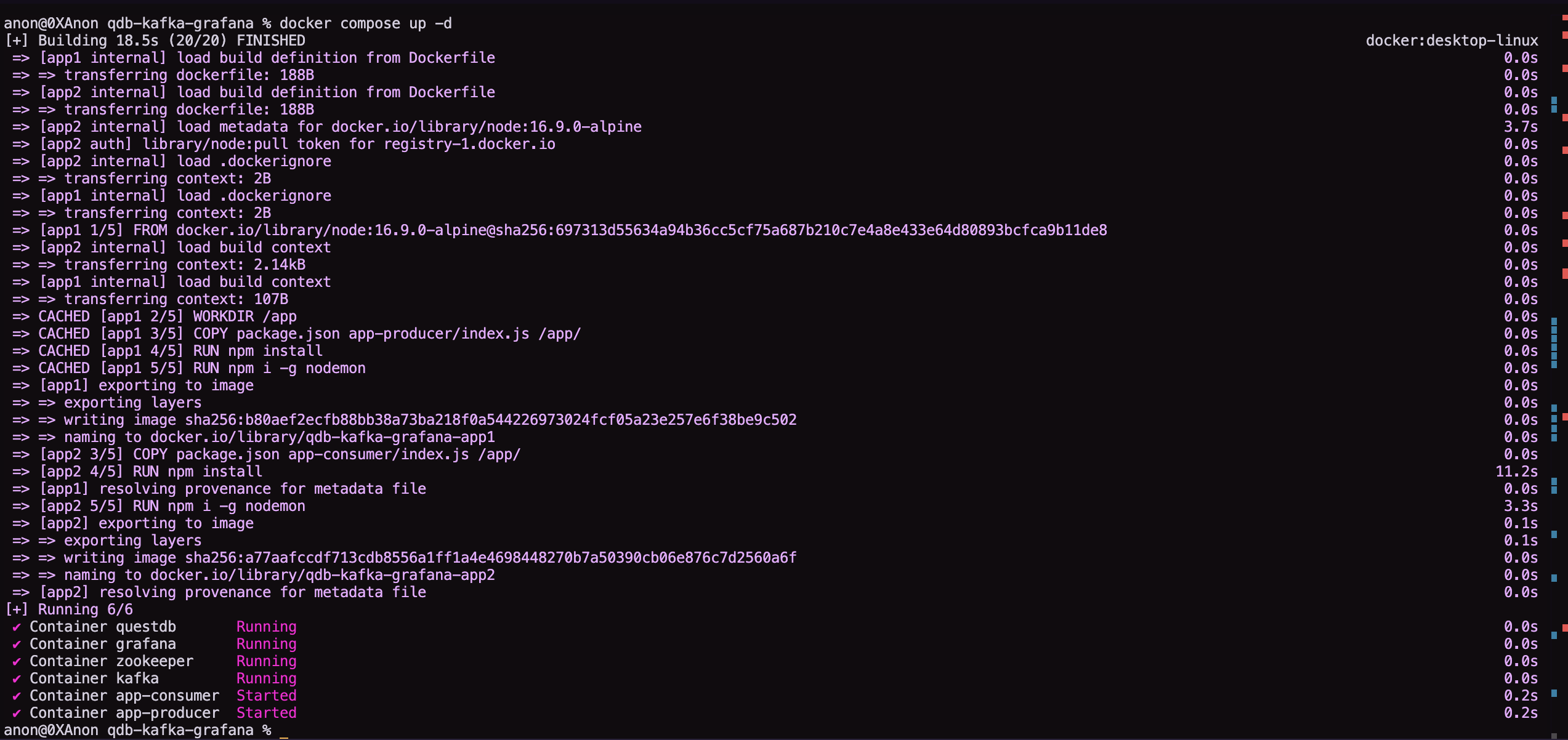
docker-compose up -d

This command will build the images and run the services in detached mode.

If all went well, you'll get a message like this that says the services are starting:

Visualizing the data with Grafana​

Raw data is interesting. But we can make it much more dynamic with a proper visualization tool. We've added Grafana, and now we can interact with our data in QuestDB. To do so, we will configure the official QuestDB data source in Grafana to visualize the data.

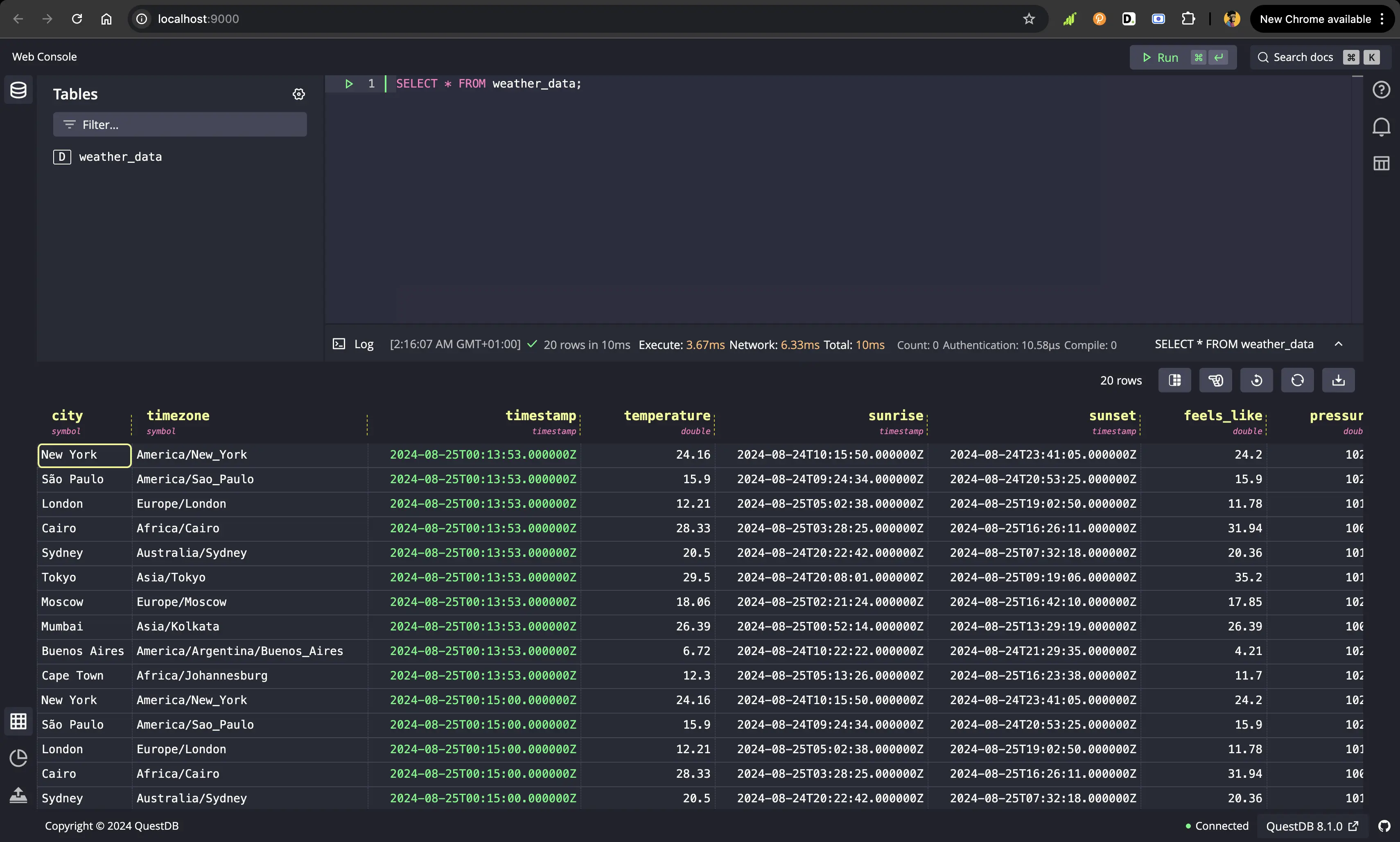
First, point your browser to the port that we set for QuestDB in the docker-compose.yml file, which is the default http://localhost:9000.

We should see the QuestDB Web Console:

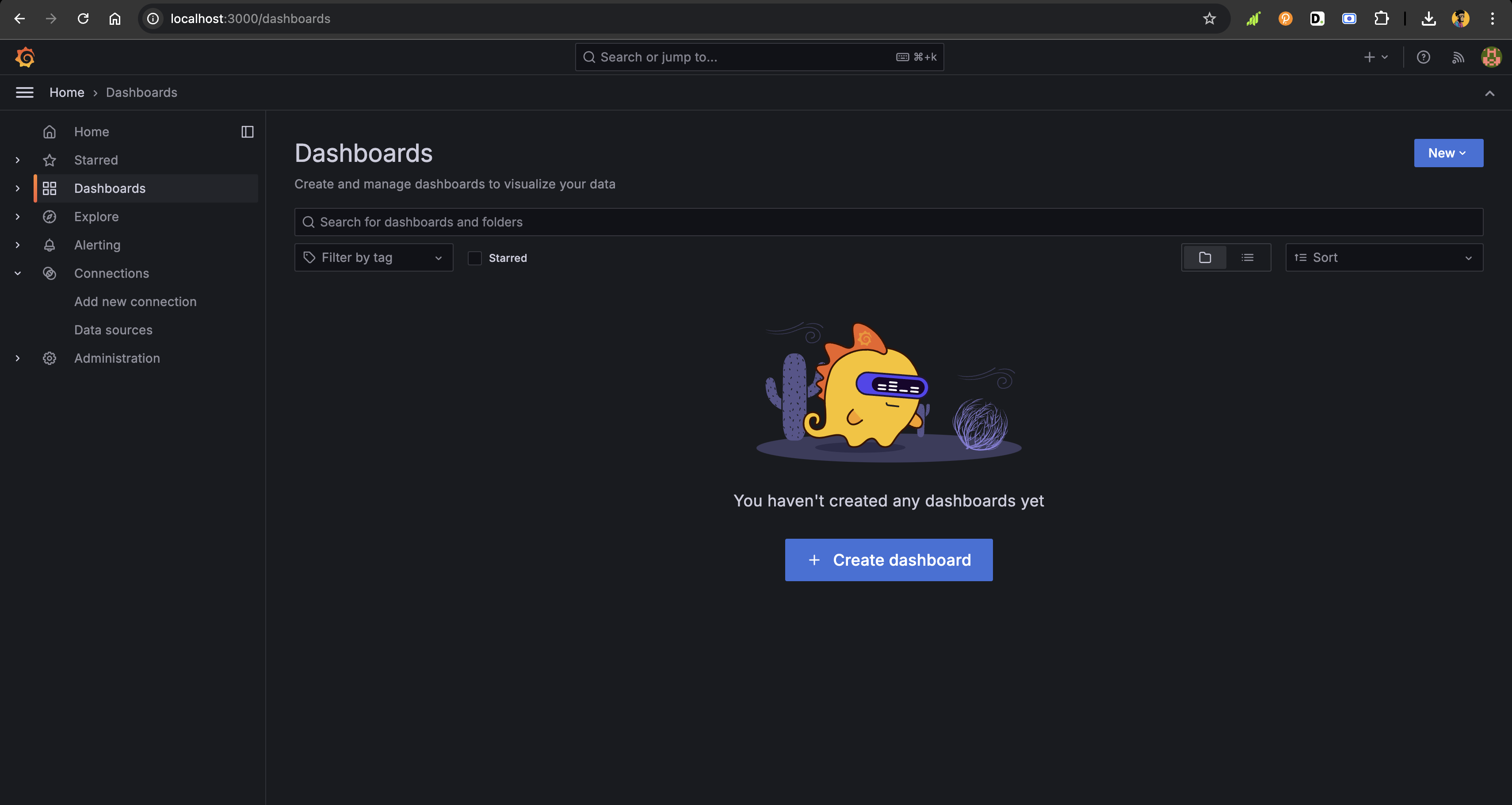
Next, access Grafana via http://localhost:3000 and log in with the default username and password, which are admin and admin respectively. For security purposes, you will be prompted to change the password, and after, you will be redirected to the Grafana dashboard:

Next, we need to create a new data source in Grafana.

Click on the Connections button on the left side of the screen.

Then click on the Add new connection button.

Now search for the QuestDB data source plugin and install it.

After installation, you will be prompted to configure it or connect it to a data source:

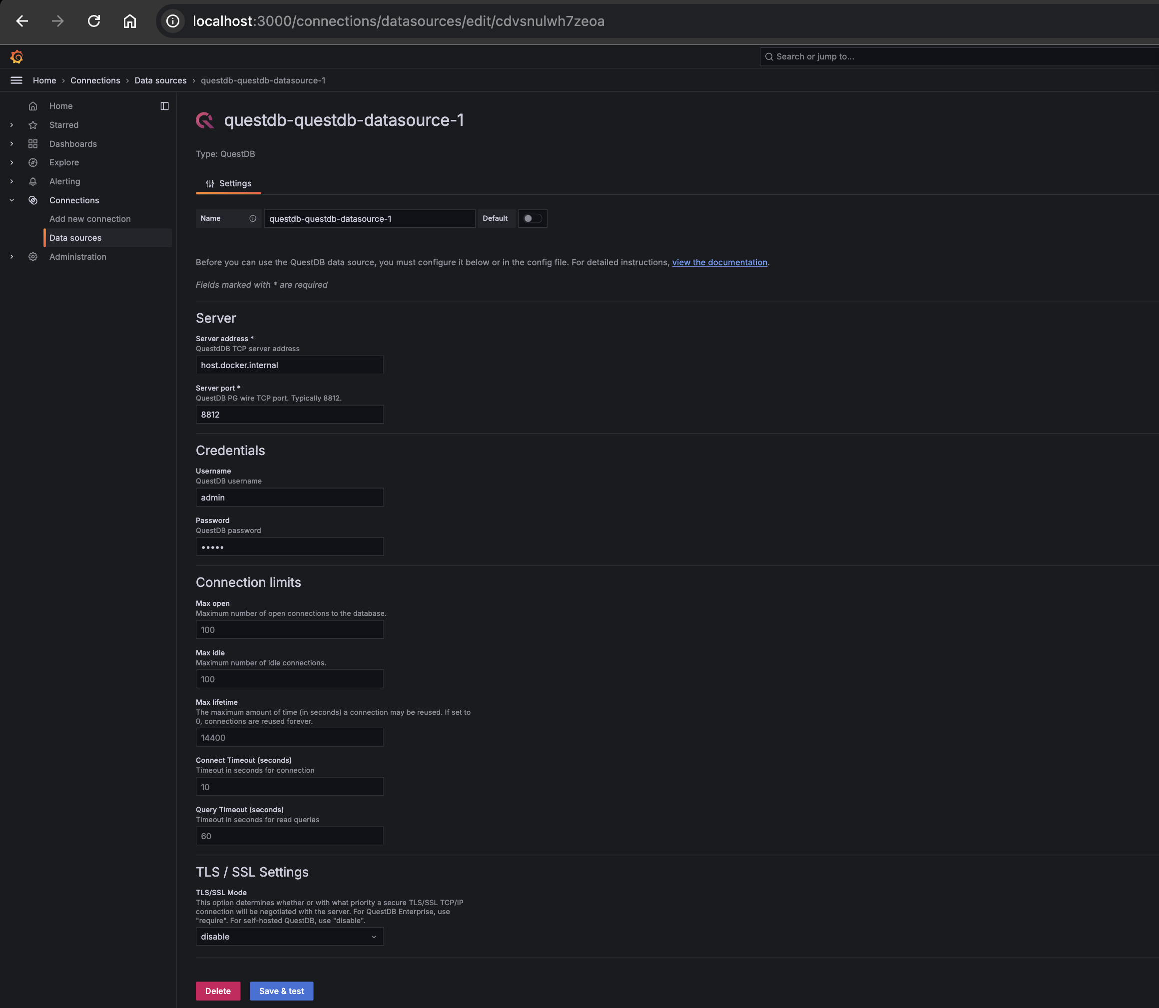
The key variables for this configuration are as follows:

Server Address: host.docker.internal
Server Port: 8812
Username: admin
Password: quest
TLS/SSL Settings: disabled

After configuring the data source, you will be prompted to save it. Click on the Save & Test button to get feedback on whether the connection is successful.

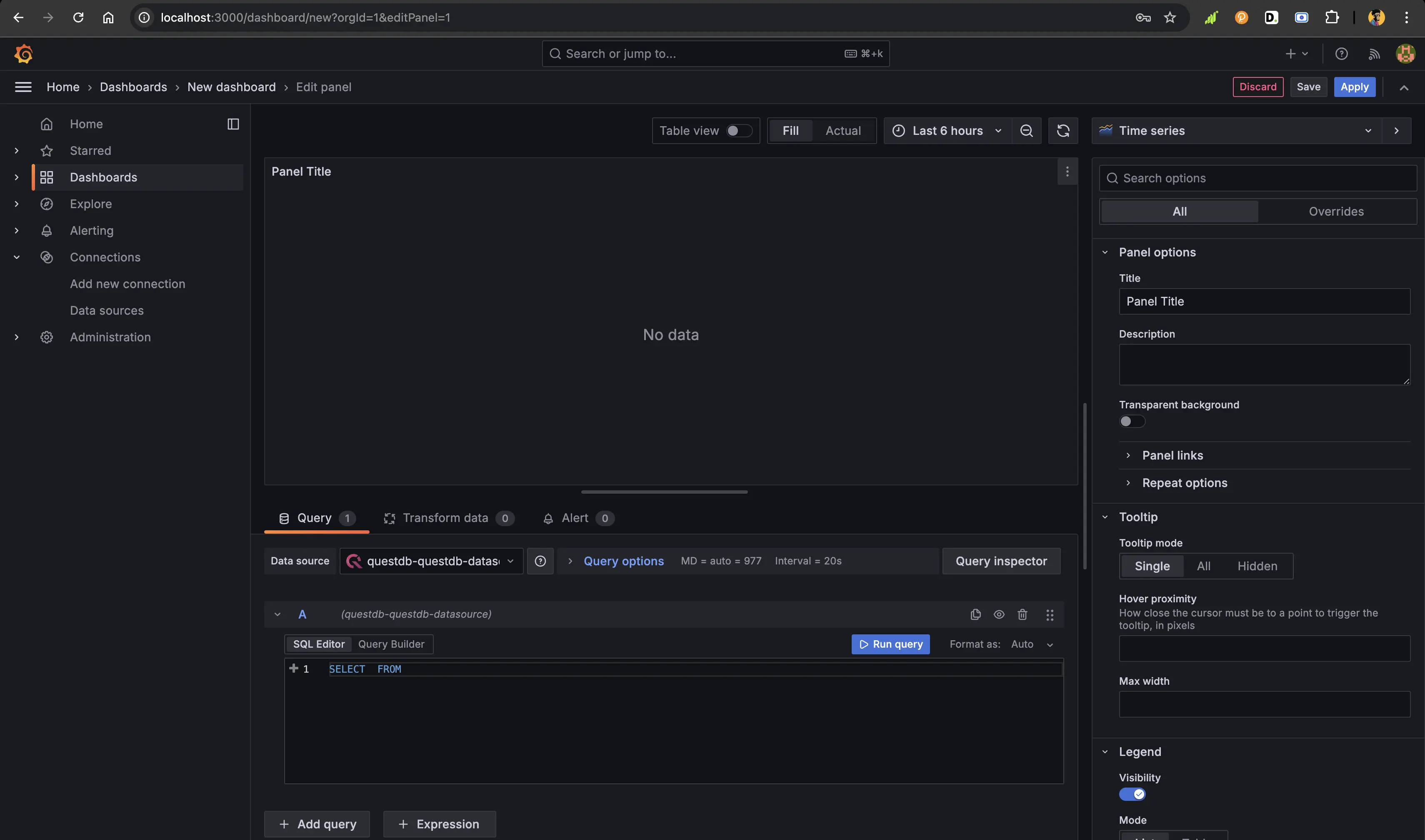
Finally, for data visualization, Click on Dashboards from the sidebar and click the Add Visualization button to start. If you are on a Grafana dashboard page with some existing dashboard visualization(s), click on the New dropdown at the top right corner of the screen.

Select the New Dashboard button, and you will be taken to the Add Visualization screen to click on it. After that, select the QuestDB data source you configured earlier, and you will be taken to where you will put your queries to start visualizing the weather data:

For the data we want to visualize, we will use a specialized query:

SELECT
   city,
   to_str(date_trunc("day", timestamp), "E, d MMM yyyy") AS current_day,
   to_str(MIN(date_trunc("hour", timestamp)), "h:mma") AS first_hour,
   to_str(MAX(date_trunc("hour", timestamp)), "h:mma") AS last_hour,
   LAST(weather_main) AS last_weather,
   CONCAT("https://openweathermap.org/img/wn/", LAST(weather_icon), "@2x.png") AS weather_icon,
   CONCAT(CAST(ROUND(AVG(temperature), 2) AS FLOAT), " °C") AS avg_temp,
   CONCAT(CAST(ROUND(AVG(feels_like), 2) AS FLOAT), " °C") AS feels_like,
   CONCAT(CAST(ROUND(AVG(pressure), 2) AS FLOAT), " hPa") AS avg_pressure,
   CONCAT(CAST(ROUND(AVG(humidity), 2) AS FLOAT), " %") AS avg_humidity
FROM weather_data
GROUP BY city, date_trunc("day", timestamp)
ORDER BY city, date_trunc("day", timestamp), first_hour

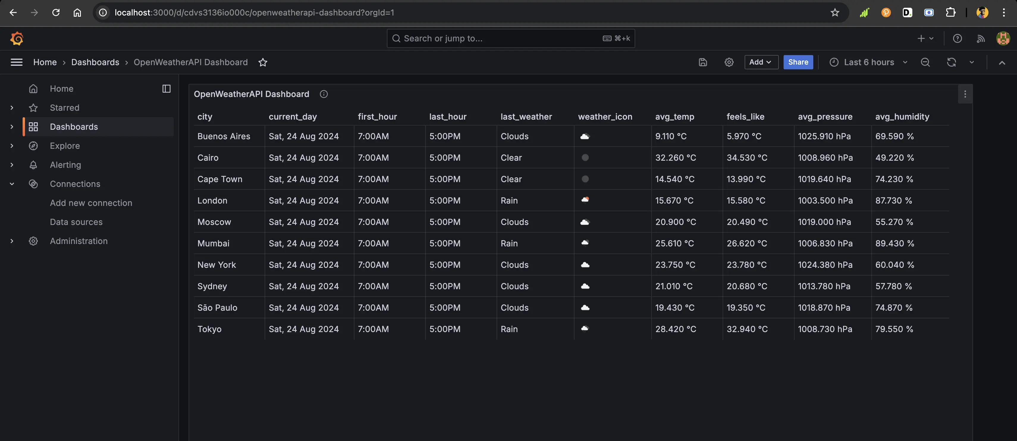
The query above will ask QuestDB to group the weather data by city and day. It will also show the first and last hour of the day for which the weather data has already been fetched. The latest weather data is shown alongside the weather icon, including average temperature, average "feels like" temperature, average pressure, and average humidity. This is the output result in the below table format.

To view this data as shown in the screenshot, use the table panel:

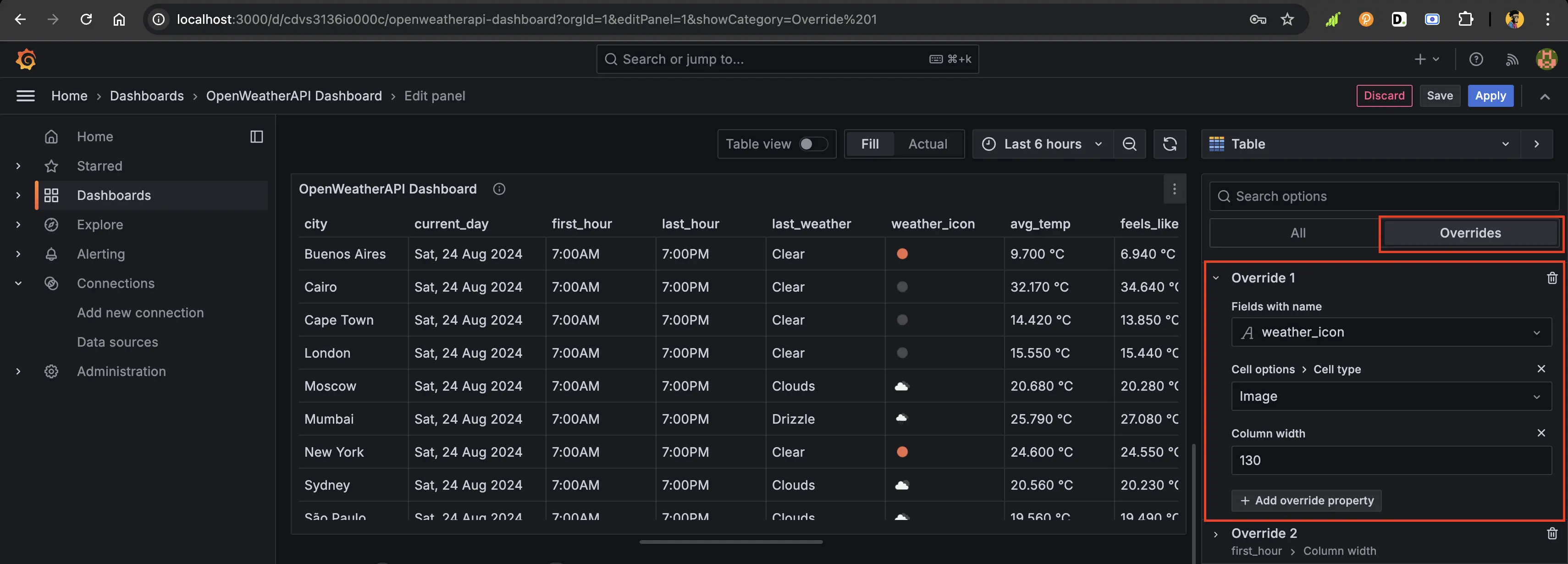
To get the weather icons as they are in the dashboard above, we can add an override for that column. To do so, click the Override section on the right-hand side of the query panel:

Wrapping up​

In this tutorial we orchestrated a microservice application together with QuestDB, Kafka, and Grafana. We also learned how to use QuestDB to store time-series data and visualize the data with Grafana. QuestDB works great on low hardware, but can scale up to massive throughput.

With this toolkit, you can ingest weather data from thousands of different sources and scale up to billions of events. Processing all these data in real-time as they come at scale can be a major challenge, and a specialized database like QuestDB can help with a lot of heavy lifting.

With respect to architecture, this tutorial is not production ready. But it is a helpful proof of concept to showcase how Kafka, QuestDB and Grafana can store and visualize different types of time-series data. And you'll also know when to bring your umbrella.