Data Lifecycle with QuestDB

Introduction#

For most applications dealing with time series data, the value of each data point diminishes over time as the granularity of the dataset loses relevance as it gets stale. For example, when applying a real-time anomaly detection model, more granular data (e.g., data collected at second resolution), would yield better results. However, to train forecasting models afterwards, recording data at such high frequency may not be needed and would be costly in terms of storage and compute.

When I was working for an IoT company, to combat this issue, we stored data in three separate databases. To show the most up to date value, latest updates were pushed to a NoSQL realtime database. Simultaneously, all the data was appended to both a time series database storing up to 3 months of data for quick analysis and to an OLAP database for long-term storage. To stop the time series database from exploding in size, we also ran a nightly job to delete old data. As the size of the data grew exponentially with IoT devices, this design caused operational issues with maintaining three different databases.

QuestDB solves this by providing easy ways to downsample the data and also detach or drop partitions when old data is no longer necessary. This helps to keep all the data in a single database for most operations and move stale data to cheaper storage in line with a mature data retention policy.

To illustrate, let’s revisit the IoT application involving heart rate data. Unfortunately, Google decided to shut down its Cloud IoT Core service, so we’ll use randomized data for this demo.

Populating heart rate data#

Let’s begin by running QuestDB via Docker:

docker run -p 9000:9000 \
-p 9009:9009 \
-p 8812:8812 \
-p 9003:9003 \
-v "$(pwd):/var/lib/questdb" \
questdb/questdb:6.5.4

We’ll create the a simple heart-rate data table with a timestamp, heart rate, and sensor ID partitioned by month via the console at localhost:9000:

CREATE TABLE heart_rate AS(
    SELECT
      x ID,
      timestamp_sequence(
        to_timestamp('2022–10–10T00:00:00', 'yyyy-MM-ddTHH:mm:ss'),
        rnd_long(1, 10, 0) * 100000L) ts,
      rnd_double(0) * 100 + 60 heartrate,
      rnd_long(0, 10000, 0) sensorId
    FROM
      long_sequence(10000000) x
    ) TIMESTAMP(ts) PARTITION BY MONTH;

We now have randomized data from 10,000 sensors over ~2 months time frame (10M data points). Suppose we are continuously appending to this dataset from a data stream, then having such frequent updates will be useful to detect anomalies in heart rate. This could be useful to detect and alert on health issues that could arise.

Downsampling the data#

However, if no anomalies are detected, having a dataset with heart rate collected every second is not useful if we simply want to note general trends over time. Instead we can record the average heart rate in one hour intervals to compact data. For example, if we’re interested in the min, max, and avg heart rate of a specific sensor, sampled every hour, we can invoke:

SELECT
    min(heartrate),
    max(heartrate),
    avg(heartrate),
    ts
FROM
    heart_rate
WHERE
    sensorId = 1000 SAMPLE BY 1h FILL(NULL, NULL, PREV);

Once you are happy with the downsampled results, we can store those results into a separate sampled_data table for other data science time to create forecasting models or do further analysis:

CREATE TABLE sampled_data (ts *timestamp*, min_heartrate *double*, max_heartrate *double*, avg_heartrate *double*, sensorId *long*) *timestamp*(ts);

INSERT INTO sampled_data (ts, min_heartrate, max_heartrate, avg_heartrate, sensorId);

SELECT ts, min(heartrate), max(heartrate), avg(heartrate), sensorId FROM heart_rate SAMPLE BY 1h FILL(NULL, NULL, PREV);

This downsampling operation can be done periodically (e.g., daily, monthly) to populate the new table. This way the data science team does not have to import the massive raw dataset and can simply work with sampled data with appropriate resolution.

Data retention strategy#

Downsampling alone, however, does not solve the growing data size. The raw sensor heart_rate table will continue to grow in size. In this case, we have some options in QuestDB to detach or even drop partitions.

Since we partitioned the original dataset by month, we have 3 partitions: 2022–10, 2022–11, and 2022–12. This can be seen under /db/heart_rate/ directories, along with other files holding metadata.

/db/heart_rate
  ├── 2022–10
  ├── 2022–11
  ├── 2022–12

After we have downsampled the data, we probably no longer need data from older months. In this case, we can DETACH this partition to make it unavailable for reads.

ALTER TABLE ‘heart_rate’ DETACH PARTITION LIST ‘2022–10’;

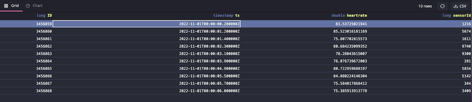
Now the 2022–10 partition is renamed to 2022–10.detached and running queries in the heart_rate table returns data from 2022–11 onwards:

SELECT * FROM ‘heart_rate’ LIMIT 10;

We can then compress this data and move it to a cheaper block storage option like S3 or GCS:

tar cfz - ‘/db/heart_rate/2022–10.detached’ | aws s3 cp - s3://my-data-backups/2022–10.tar.gz

If we need to restore this partition for further analysis, we can re-download the tar file to a new directory named PARTITION-NAME.attachable under /db/ (or where the rest of the QuestDB data lives) and uncompress the tar file:

mkdir 2022–02.attachable | aws s3 cp s3:/my-data-backups/2022–10.tar.gz - | tar xvfz - -C 2022–10.attachable - strip-components 1

With the data in place, simply use the ATTACH command:

ALTER TABLE heart_rate ATTACH PARTITION LIST ‘2022–10’;

We can verify the partition has been attached back by running the count query and seeing 10M records:

SELECT count() FROM heart_rate;

Alternatively, if we want to simply delete partitions, we can use the DROP command to do so. Unlike the DETACH command, this operation is irreversible:

ALTER TABLE heart_rate DROP PARTITION LIST ‘2022–10’;

Blasting fast ingest. SQL analytics. $200 in free credit.