Analyzing multi-stream market data with Databento, Grafana and QuestDB

Market data comes in droves and can be very difficult to manage. This is true for those who interface with a single financial exchange, let alone many. Banks, hedge funds, and other groups trying to multiple wrangle capital markets have their hands full.

That's why services like Databento - market data aggregator - are valuable. They provide a single, normalized feed that covers multiple venues. This convenience comes with some tradeoffs, but for the most part Databento maintains the three financial connectivity ideals of latency, convenience, and integrity. And the best part? It interfaces well with QuestDB for aggregation and analysis.

In this post, we'll look at Databento and see how to get started pulling live prices into QuestDB.

What are market data aggregators?

In past articles, we looked at building live trading dashboards to better understand markets in real-time using data from crypto exchanges such as Coinbase public API. While it was trivial to connect to a single exchange, in a real trading setup, one would need to establish and maintain connections with multiple venues, all with their own standards.

Market data aggregators are set to solve this problem in both crypto and tradfi. They take away the pain of onboarding and maintaining multiple exchange connections by providing a single normalised feed that covering multiple venues.

Some aggregators pass through raw market data directly from the exchanges. This typically induces lower latency but lacks standardisation. It's simple to tap into the aggregator's feed, but then there is downstream work to account for each underlying venue's specifics such as trading phases.

Other aggregators may offer a very standardised REST API where all market data is normalised. However, this is often at the expense of latency and integrity. Such services often discard some of the data that does not fit their model, resulting in less granular information for downstream consumers.

About Databento

Databento strikes us with their commitment to maintain the three ideals of latency, convenience, and integrity. The engineering team comprises former high-frequency trading tech engineers who have been dealing with the challenges of market data throughout their careers. The engineering effort that went into the solution is very apparent from a glance at the documentation.

The product is very feature rich, so we'll just provide a brief summary:

• Covers both live and historical market data
• Covers the main exchanges such as NYSE, NASDAQ, OPRA, and the CME.
• Multiple clients available such as Python, C++, and an HTTP API.

One key feature is the choice of schemas to fit each individual's granularity needs:

• Quote-based schemas
  • MBO: Market by order. The most granular service, showing each individual order. This is often called 'L3'
  • MBP-10: Market depth up top a given level (e.g. 10 orders). This is often referred to as 'L2'
  • MBP-1: Top of book or 'L1', i.e. best bid and offer
• Trades based schemas
• Aggregates, such as per minute, per second, and so on
• Other specialised schemas suuch as statistics, and auction data.
• Both historical and live market data covering the largest exchanges such as NYSE, NASDAQ, the CME and OPRA

Getting started in Python

To demonstrate, we'll setup a market data ingestion pipeline using the Databento Python client connected into a QuestDB back-end. We'll then use this to ingest data, visualise it in Grafana, and calculate derived data and metrics to better understand the markets.

Pre-requisites

To complete this tutorial we need the following running:

• QuestDB server
• Grafana server

We'll also need a working Python environment with the following libraries:

• Databento python client
• QuestDB Python client

The libraries can easily be installed as follows:

pip3 install questdb
pip3 install databento

Creating a Databento client

When signing up with Databento, whether with a trial or a live account, you will be given an API_KEY. The key allows you to identify your requests and will be used to calculate your consumption if you are on a metered plan. The key looks like the following: db-abcdefGHIJKLmno123456789

The first step consists of creating a client with your key:

db_client = db.Live(key="YOUR_API_KEY")

Creating a Databento subscription

After creating your client, you can create a market data subscription. There is a whole set of parameters allowing you to create a custom subscription. Checkout the official documentation for all the available parameters.

For our purposes, we will create a subscription for the CME S&P 500 E-Mini futures for June 24 maturity:

db_client.subscribe(
    dataset="GLBX.MDP3",
    schema="mbp-1",
    stype_in="raw_symbol",
    symbols="ESM4",
)

Note the following parameters:

• dataset: Identifier for the dataset, in this instance Globex.
• schema: The data schema we want to subscribe to. This schema depends on the individual needs. In this instance, we're using the mbp-1 schema, also known as L1 or top-of-book.
• stype_in: The symbology type of the instrument identifier.
• symbols: The symbol(s) we want to subscribe to. You can use ALL_SYMBOLS to subscribe to all, a list of symbols, or a single symbol as we did in this example.

Accessing records

The Databento client offers synchronous and asynchronous iterators allowing us to easily churn through returned records. We can use this in a simple form to just print the records we're getting:

for record in db_client:
  print(record)

SymbolMappingMsg { hd: RecordHeader { length: 44, rtype: SymbolMapping, publisher_id: 0, instrument_id: 5602, ts_event: 1716651181749148284 }, stype_in: RawSymbol, stype_in_symbol: "ESM4", stype_out: InstrumentId, stype_out_symbol: "ESM4", start_ts: 18446744073709551615, end_ts: 18446744073709551615 }
Mbp1Msg { hd: RecordHeader { length: 20, rtype: Mbp1, publisher_id: GlbxMdp3Glbx, instrument_id: 5602, ts_event: 1716555600001896245 }, price: 5300.500000000, size: 1, action: 'C', side: 'A', flags: 0b10000010, depth: 0, ts_recv: 1716555600002029557, ts_in_delta: 13676, sequence: 31295832, levels: [BidAskPair { bid_px: 5300.250000000, ask_px: 5300.500000000, bid_sz: 29, ask_sz: 23, bid_ct: 17, ask_ct: 15 }] }
Mbp1Msg { hd: RecordHeader { length: 20, rtype: Mbp1, publisher_id: GlbxMdp3Glbx, instrument_id: 5602, ts_event: 1716555600002031293 }, price: 5300.250000000, size: 1, action: 'A', side: 'B', flags: 0b10000010, depth: 0, ts_recv: 1716555600002145155, ts_in_delta: 12998, sequence: 31295840, levels: [BidAskPair { bid_px: 5300.250000000, ask_px: 5300.500000000, bid_sz: 30, ask_sz: 23, bid_ct: 18, ask_ct: 15 }] }
Mbp1Msg { hd: RecordHeader { length: 20, rtype: Mbp1, publisher_id: GlbxMdp3Glbx, instrument_id: 5602, ts_event: 1716555600002147871 }, price: 5300.250000000, size: 1, action: 'A', side: 'B', flags: 0b10000010, depth: 0, ts_recv: 1716555600002259523, ts_in_delta: 14584, sequence: 31295852, levels: [BidAskPair { bid_px: 5300.250000000, ask_px: 5300.500000000, bid_sz: 31, ask_sz: 23, bid_ct: 19, ask_ct: 15 }] }
Mbp1Msg { hd: RecordHeader { length: 20, rtype: Mbp1, publisher_id: GlbxMdp3Glbx, instrument_id: 5602, ts_event: 1716555600005726245 }, price: 5300.250000000, size: 1, action: 'T', side: 'A', flags: 0b00000000, depth: 0, ts_recv: 1716555600005967117, ts_in_delta: 15150, sequence: 31295917, levels: [BidAskPair { bid_px: 5300.250000000, ask_px: 5300.500000000, bid_sz: 31, ask_sz: 23, bid_ct: 19, ask_ct: 15 }] }
Mbp1Msg { hd: RecordHeader { length: 20, rtype: Mbp1, publisher_id: GlbxMdp3Glbx, instrument_id: 5602, ts_event: 1716555600005726245 }, price: 5300.250000000, size: 1, action: 'M', side: 'B', flags: 0b10000010, depth: 0, ts_recv: 1716555600005973943, ts_in_delta: 12710, sequence: 31295918, levels: [BidAskPair { bid_px: 5300.250000000, ask_px: 5300.500000000, bid_sz: 30, ask_sz: 23, bid_ct: 19, ask_ct: 15 }] }

In response, we get several types of messages. SymbolMappingMsg records are providing us with initial reference data information. Mbp1Msg records are supplying market-data events, in this case updates in the top-of-book.

In this instance we're only looking to record market-data events so we'll add a branch to only account for the type of message received:

for record in db_client:
  if isinstance(record, db.MBP1Msg):
    print(record)

Accessing records elements

Since we're using the Mbp1 schema, we can refer to the associated documentation to understand how to access record elements.

In this instance we are interested in the following basic fields:

• bid_sz and ask_sz
• bid_px and ask_px
• ts_event

Since we're looking at an orderbook object (though limited to the top of the book) we need to specify the orderbook level we want for each field. In this case, it is 0. So, for example this means we set following:

bid_size_level_0 = record.levels[0].bid_sz
bid_price_level_0 = record.levels[0].bid_px

In addition, the prices are supplied as integer numbers to avoid decimals. This means that to get the quoted price, we need to scale the price using an 1e-9 multiplier:

bid_price_level_0 = record.levels[0].bid_px * 0.000000001

If we use all of the above, we can start printing string representations of the top-of-book in our console:

import databento as db
import pandas as pd

db_client = db.Live(key="YOUR_API_KEY")
db_client.subscribe(
    dataset="GLBX.MDP3",
    schema="mbp-1",
    stype_in="raw_symbol",
    symbols="ESM4",
)

for record in db_client:
    if isinstance(record, db.MBP1Msg):
        bid_size = record.levels[0].bid_sz
        ask_size = record.levels[0].ask_sz
        bid_price = record.levels[0].bid_px*0.000000001
        ask_price = record.levels[0].ask_px*0.000000001
        ts = pd.to_datetime(record.ts_event, unit='ns').strftime('%H-%M-%S.%f')
        print(f'{ts}\t {bid_size} \t {bid_price} - {ask_price} \t {ask_size}')

The console output should look as follows:

Ingesting into QuestDB

At this stage we are able to establish a live connection to market data and access the record elements such as prices, sizes and timestamps. We can now start ingesting this into QuestDB to visualise in realtime in Grafana, calculate derived metrics and do some analysis.

To ingest into QuestDB we'll need to:

• Setup a configuration string
• Create an instance of a sender from this configuration string
• Create and send records

A simple strawman example looks like the following. The only particularity is that we need to convert the timestamp from the record to make it consistent with the exchange timestamp instead of using the server timestamp with TimestampNanos.now() for example:

questdb_conf = "http::addr=localhost:9000;username=admin;password=quest;"
with Sender.from_conf(questdb_conf) as sender:
  sender.row(
    'top_of_book',
    symbols={'instrument': 'ESM4'},
    columns={'bid_size': record.levels[0].bid_sz,
             'bid': record.levels[0].bid_px*0.000000001,
             'ask': record.levels[0].ask_px*0.000000001,
             'ask_size': record.levels[0].bid_sz},
    at=np.datetime64(record.ts_event, 'ns').astype('datetime64[ms]').astype(object))
  sender.flush()

Subscribing to multiple instruments

In the past sections we set up the building blocks for our ingestion pipeline. We can now use these blocks to, for example, ingest all the S&P futures from the CME.

To do this, we'll change a few things and first expand our universe of symbols to ES.FUT which will cover all E-Mini SP500 futures, including rolls. We also need to modify our ingestion script to parse the initial symbology so that the numerical instrument_id (for example 46995) be corrected to the appropriate trading symbol (for example ESM4).

We can do this by building a dictionary using the SymbolMappingMsg records, and then access this dictionary to fetch the corresponding trading symbol:

# First we build up the static data dictionary
instruments = {}
if isinstance(record, db.SymbolMappingMsg):
    instruments.update({record.hd.instrument_id : record.stype_out_symbol})

# Second, we access this dictionary to get the corresponding trading symbol
instrument = instruments[record.instrument_id]

Having done all this we can launch our ingestion and start setting up a few views in Grafana using QuestDB SQL.

Creating a dashboard

It is a good idea to create Grafana variables when ingesting several instruments into the same table. In this case, let's create a symbol variable.

This allows the following:

• Get the list of available symbols automatically from the database
• Use the generic $symbol in queries, which will automatically be replaced by the selected values in the dashboard
• Use the repeat functionality to create multiple charts from one template.

Learn more about Grafana symbols in our blog on symbol management.

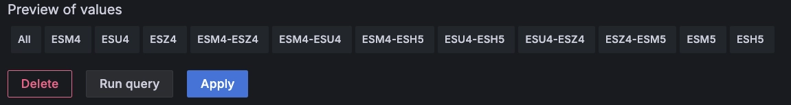
Since the list of symbols is dynamic, we can use the Query variable type with the following definition:

SELECT DISTINCT instrument FROM market_data

We can see a preview of values on the variable definition screen in Grafana which shows we did a successful setup:

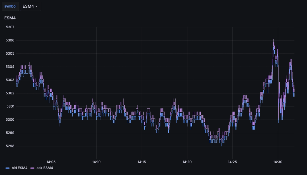
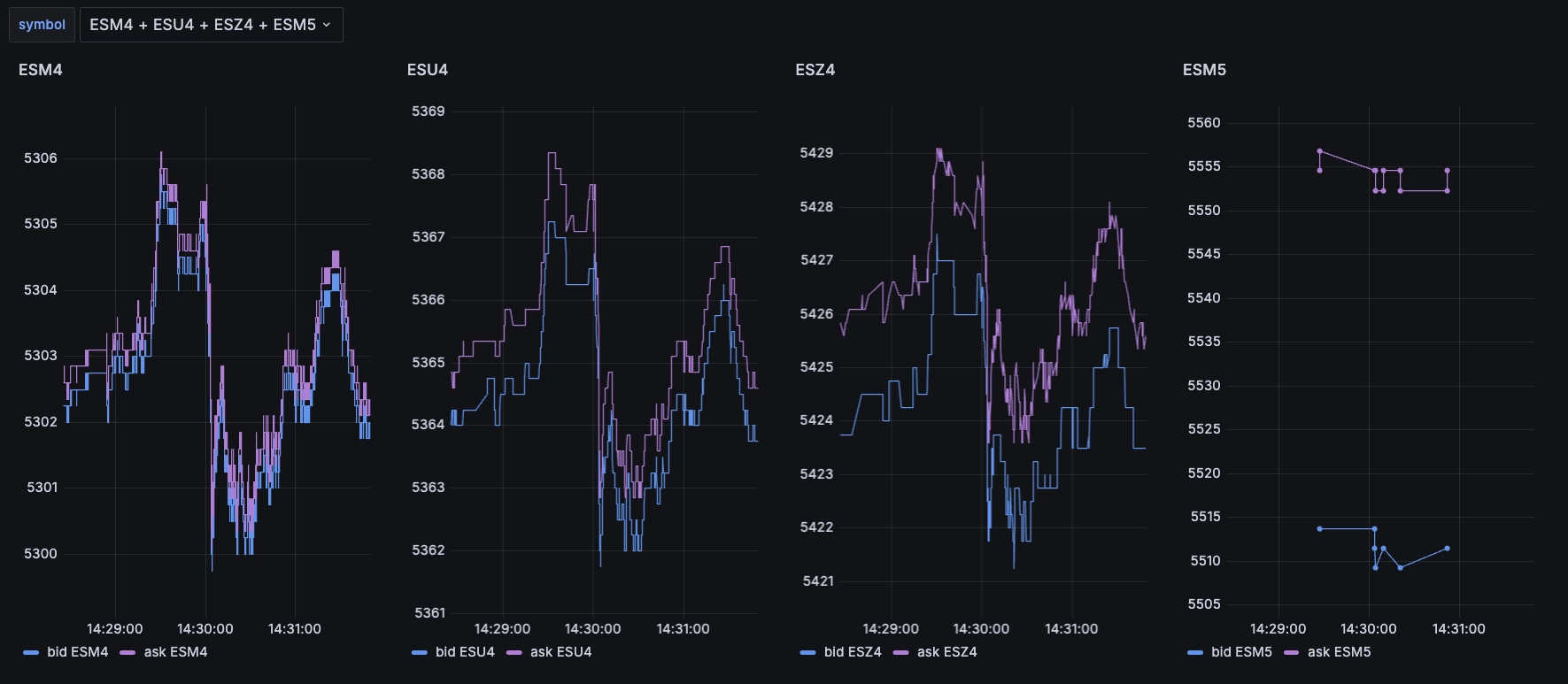
We can now create some charts. Note the use of the freshly-created $symbol Grafana variable:

SELECT timestamp, instrument, bid, ask
FROM market_data
WHERE $__timeFilter(timestamp) AND instrument = $symbol

This variable allows us to change the instrument on the fly using the top-left dropdown:

One nice thing about Grafana are the Repeat options. With them, you can duplicate panels dynamically based on your selected instruments of interest. After setting up a variable as we did for $symbol you can use it to create other charts on the fly:

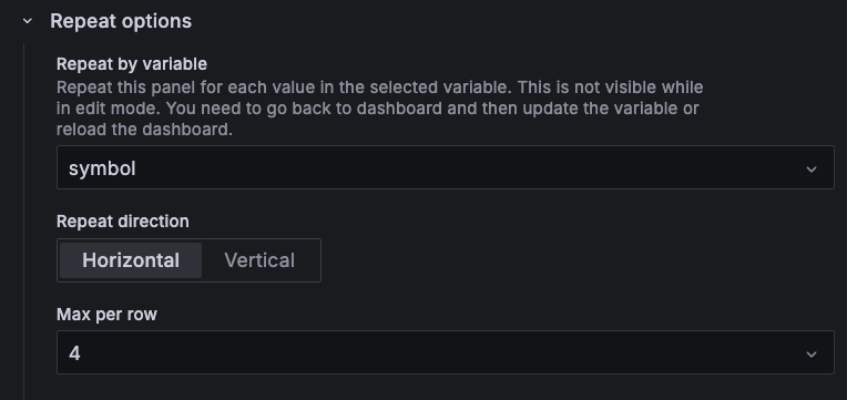
Using this, we can easily display the prices for the upcoming S&P futures expiries:

Deriving metrics

Above, we gathered market data and displayed it in a Grafana dashboard. However, we are missing one important dimension which consists of the derived relationships between the prices of different instruments.

While we are only looking at top-of-book in this example, there is already room to derive interesting metrics that allow us to make more sense of the markets.

Before we go on, let's quickly explain the financial concept of a "roll" for those who are unfamiliar.

Rolling into it

In finance, a "roll" refers to the process of closing out a position in a futures contract that is nearing its expiration and simultaneously opening a new position in a futures contract with a later expiration date. This is done to maintain a continuous exposure to the underlying asset or market without having to take physical delivery or settle the contract.

The difference in price between the expiring contract and the new contract reflects factors such as the cost of carry, interest rates, and expectations about future market conditions. The process of rolling futures contracts is common among traders and investors who want to maintain their positions over a longer period without interruption.

For example, if an investor holds a long position in the September futures contract for the S&P 500 and wants to maintain this position into December, they would sell the September contract and buy the December contract. The price difference between these contracts, known as the "roll yield," can be positive or negative depending on market conditions.

Looking at liquidity

We can use the following query to look at the bid-ask spread, in basis points, of the outright futures (i.e. excluding rolls) until the end of 2024:

SELECT timestamp, instrument, (ask-bid)/((bid+ask)/2) * 10000 spread_bps
FROM market_data
WHERE $__timeFilter(timestamp)
AND instrument LIKE 'ES%4'
AND NOT instrument LIKE '%-%'

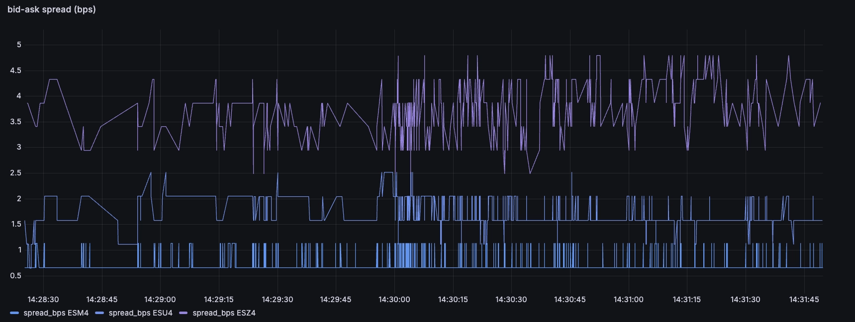
A few noteworthy observations:

• The futures are extremely liquid. The bid-ask on the front-month is less than one basis points, that's less than 1% of 1%, i.e < 0.01%
• The subsequent futures are less liquid, but still very tight (around 2 basis points for the next maturity, and 3.5 for the subsequent one)
• The small transient jumps in spread likely correspond to trades whereby an incoming order takes out the quantity at the top-of-book. There is a short amount of time where the book is slightly wider as a result, until the contracted market-marker refills their quotes

Many of these markets have dedicated market-makers who have quoting obligations. For example, they will show a minimum size for a maximum spread X% of the time. These obligations ensure consistent liquidity and tight spreads, contributing to market efficiency.

The commercials vary by exchange, but typically such market-markers are either directly paid by the exchange, or indirectly paid in the form of rebates on their trading fees.

Such rebates are contingent, and sometimes somewhat proportional to the fulfilment of obligations, or to the percentage of volume traded by the different market-makers. This explains the steadiness of the bid-ask spreads above: the bid-ask spreads tend to be constant for a given instrument under normal market conditions as market-makers try to fulfil their obligations.

However, the spread alone does not fully give us an idea of the liquidity. We also need to look at the sizes. In fact, top-of-book also gives a very partial view of the liquidity situation, but it's good enough to have a rough idea of the dynamics.

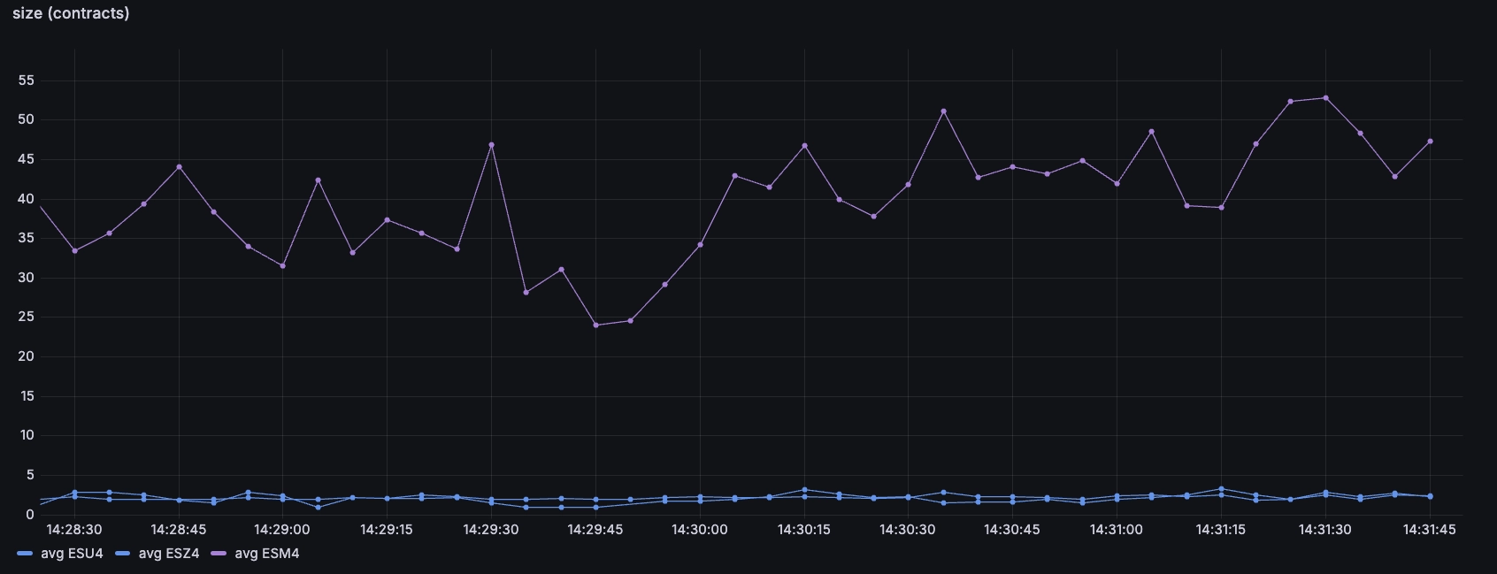
We can adapt our query to look at the minimum size quoted on the three above contracts, and this gives us another dimension:

SELECT timestamp, instrument, avg(case when ask_size > bid_size then bid_size else ask_size end)
FROM market_data
WHERE $__timeFilter(timestamp)
AND instrument LIKE 'ES%4' AND NOT instrument LIKE '%-%'
SAMPLE BY 5s

With only a few basis points spread, it may have seemed like the three contracts were extremely liquid. But it turns out that when looking at size, the front-month ESM4 has significantly more size than the back-month instruments:

What typically tends to happen here is that as the expiry of the 'active' contract approaches, and then participants roll their contracts to the next maturity. So in this example, they will sell the June M futures and buy September U. This is done through the use of 'roll' instruments which represent the atomic trading of both legs.

Looking at rolls

We can see the rolls market using instruments such as ESM4-ESU4. When you 'buy' the roll instrument, it means you are simultaneously buying the September and selling the June futures:

This shows us that the 'cost of roll' is around 62, which means for each underlying index you would 'pay' $62. The futures correspond to a given number of indexes which depend on their specs, and therefore one can 5x this for the mini contract which represents 5 indexes.

This difference represents the difference in cost of carry for rolling the position for another three months. We can estimate this cost roughly as follows:

The cost of carry is a function of mostly two things:

• The interest cost to borrow money to buy the underlying stocks
• The dividends one expects to receive from these stocks, because the dividends are not reinvested in the index

We can see here the impact of Covid, inflation, and FED policy. The interest rates are about 5% per annum in the US, and that explains most of the cost of carry above.

We can close this post by using all of our data to calculate the implicit roll cost between the different contracts. We can then derive the implicit annualised cost of holding a position.

Normally, we would calculate this based on spot index, but in this case -- to simplify -- we'll assume that the front-month is spot as it will expire in a few weeks:

WITH
M AS (SELECT timestamp, instrument, (bid + ask)/2 mid_M FROM SP_FUTURES WHERE $__timeFilter(timestamp) AND instrument = 'ESM4'),
U AS (SELECT timestamp, instrument, (bid + ask)/2 mid_U FROM SP_FUTURES WHERE $__timeFilter(timestamp) AND instrument = 'ESU4'),
Z AS (SELECT timestamp, instrument, (bid + ask)/2 mid_Z FROM SP_FUTURES WHERE $__timeFilter(timestamp) AND instrument = 'ESZ4')

SELECT
  M.timestamp,
  (mid_U/mid_M-1)*10000*4 implicit_carry_june_sep,
  (mid_Z/mid_M-1)*10000*2 implicit_carry_dec_sep
FROM M ASOF JOIN U ASOF JOIN Z

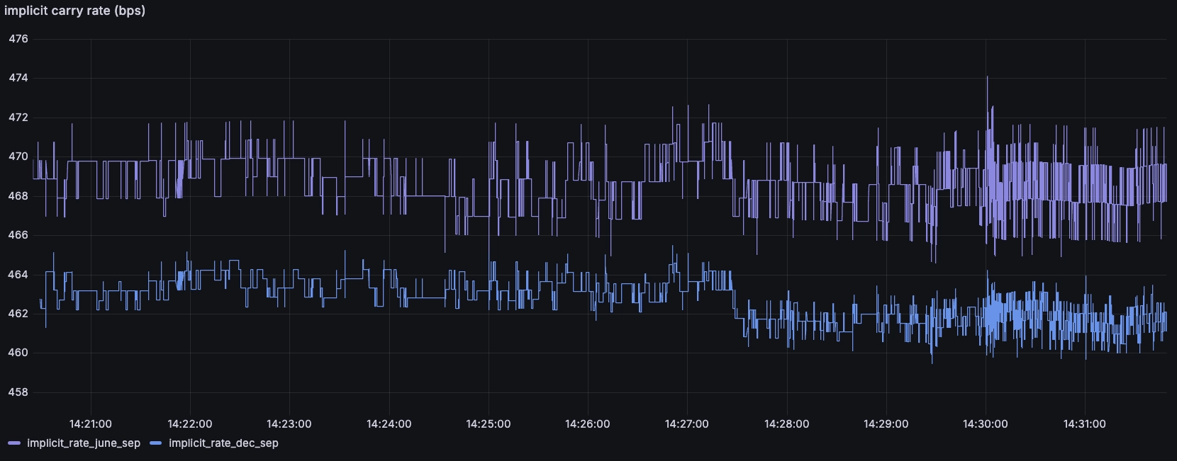
We can see the rates are quite similar, with the implicit annual rate for the December maturity lower than the September. This is likely because the extra time to maturity means more dividends falling out of the underlying stocks.

Conclusion

We did a lot in this post. We gathered market-data via Databento which was a breeze, collected it in a QuestDB instance, setup some Grafana dashboards, and ran some derived analyses with SQL. If you are looking to ingest market-data, or compute simple analytics like the above, or more complex ones, please do get in touch!

Working on anything intersting in finance? Have any questions?

Swing by our Community Forum to learn more.