Create an ADS-B flight radar with QuestDB and a Raspberry Pi

We've been keen on the Raspberry Pi lately. It's fun to play with and makes for an excellent demonstration. The Pi shows us that even with minimal hardware we can create useful and scaleable things.

In our previous post, we showed how to setup a lightweight QuestDB server on a Raspberry Pi. In this post, we'll use the same server, only juiced up with a little more sensor hardware.

Our mission? To track airplanes flying around the world. We'll apply a similar method used by FlightRadar24, FlightAware, and other flight tracking services that use the ADS-B service.

What is ADS-B?​

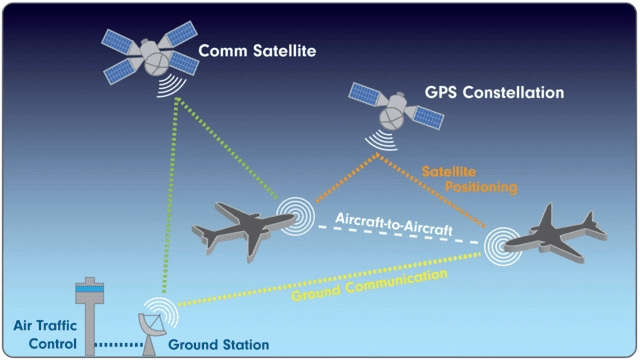
ADS-B is an acronym for Automatic Dependent Surveillance Broadcast.

Aircraft equipped with this system automatically broadcast their position, identification, bearing, altitude, and more, at a regular interval to nearby aircraft and ground stations. These ground stations are vital to keep our skies safe. And we're about to build one.

The system is called 'dependent' because the transmitted position is calculated using the aircraft's onboard navigation systems, which often includes GPS, inertial navigation units, and more.

In other words, the position transmitted is where the aircraft "thinks" it is. It supplements radar in Air Traffic Control situations, and can also help aircraft identify each other's relative positions.

If you're a frequent reader of the blog, you'll notice this is similar to the AIS system for ships we discussed in Tracking sea faring ships.

Required gear​

To track planes, we need additional hardware beyond the base QuestDB + Raspberry Pi IoT server.

We need:

• An ADS-B SDR dongle. In this case, we'll use the FlightAware prostick.
• A 1090MHz SDR antenna. These come either for indoor or outdoor use. The one we'll use is similar to this.
• Optionally, a filter which will help clean up the signals and improve reception in crowded areas with a lot of signal interference.

To capture data, we'll use a fork of dump1090 from FlightAware. Dump1090 decodes the flight information that we receive via our antenna. To do so, it leverages the ADS-B dongle to relay the latest aircraft positions into a .json file.

This is enabled via a process called RTL-SDR. RTL-SDR refers to a software-defined radio (SDR) system that utilizes inexpensive DVB-T antenna based on the RTL2832U chipset.

Now, let's install the software.

Installation​

To build our monitoring station, we follow this great tutorial with a few tweaks:

sudo apt update && sudo apt upgrade
sudo apt install git-core git cmake build-essential libusb-1.0-0-dev
git clone https://github.com/osmocom/rtl-sdr.git
cd rtl-sdr && mkdir build && cd build && cmake  ../ -DINSTALL_UDEV_RULES=ON && make && sudo make install

What's up here? First, we get the antenna going:

1. sudo apt update && sudo apt upgrade

   • sudo apt update: Fetches the list of available updates.
   • sudo apt upgrade: Upgrades all the installed packages to the latest version.

2. sudo apt install git-core git cmake build-essential libusb-1.0-0-dev

   • git-core and git: Version control systems used to manage the source code.
   • cmake: A cross-platform tool to manage the build process.
   • build-essential: Oncludes a compiler and libraries essential for compiling C/C++ programs.
   • libusb-1.0-0-dev: Development files for the libusb library, used for USB device access.

3. git clone https://github.com/osmocom/rtl-sdr.git

   • Clones the repository containing the RTL-SDR source code into a directory named rtl-sdr.

4. cd rtl-sdr && mkdir build && cd build && cmake ../ -DINSTALL_UDEV_RULES=ON && make && sudo make install

   • Changes directory to the cloned rtl-sdr folder, creates a new directory named build for an out-of-source build, changes into this build directory, configures the project with cmake, compiles it with make, and then installs it using sudo make install.
   • The -DINSTALL_UDEV_RULES=ON option tells cmake to configure the build to install udev rules, which are needed for non-root access to the USB device.

Next, we install and build dump1090:

git clone https://github.com/flightaware/dump1090
sudo apt-get install build-essential fakeroot debhelper librtlsdr-dev pkg-config libncurses5-dev libbladerf-dev libhackrf-dev liblimesuite-dev libsoapysdr-dev
./prepare-build.sh bullseye    # or buster, or stretch
cd package-bullseye            # or buster, or stretch
dpkg-buildpackage -b --no-sign

And what's happening here? We're preparing dump1090

1. git clone https://github.com/flightaware/dump1090

   • Clone the dump1090 source code, which decodes radio transmission data from aircraft, into a directory named dump1090.

2. sudo apt-get install build-essential fakeroot debhelper librtlsdr-dev pkg-config libncurses5-dev libbladerf-dev libhackrf-dev liblimesuite-dev libsoapysdr-dev

   • Installs additional packages and libraries needed to compile and run dump1090:
     • fakeroot: Simulates superuser privileges.
     • debhelper: Collection of programs and scripts to automate the creation of Debian packages.
     • librtlsdr-dev: Development files for the RTL-SDR library.
     • pkg-config: Manages compile and link flags for libraries.
     • libncurses5-dev: Library for ncurses, which is used for terminal handling.
     • libbladerf-dev, libhackrf-dev, liblimesuite-dev, libsoapysdr-dev: File for various SDR hardware platforms.

3. ./prepare-build.sh bullseye (or buster, stretch)

   • Executes the prepare-build.sh script with a parameter specifying the Debian version (bullseye, buster, or stretch).

4. cd package-bullseye (or buster, stretch)

   • Changes directory to the one prepared for the specific Debian release.

5. dpkg-buildpackage -b --no-sign

   • Builds the dump1090 package from the source without signing the package. The -b option tells dpkg-buildpackage to build the binary package only.

That'll do it!

Start monitoring​

With everything installed, connect the dongles and run the utilities!

The system generally requires line-of-sight. To maximise signal reception, mount the antenna as high as possible with a clear view of the sky. And preferably outside, where the airplanes are.

Let's navigate to our dump1090 build directory.

We'll use the Bullseye Raspbian release:

cd dump1090/package-bullseye

We can then activate monitoring with a few options:

./dump1090 --interactive --net --stats --stats-range --write-json ~/aircraft

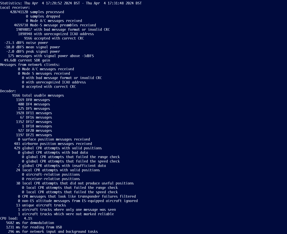
• --interactive: Displays the currently visible aircraft in the terminal
• --net: Opens a web server on localhost:8080 where we can see the surrounding aircraft
• --stats: Displays some statistics when you close the process
• --write-json ~/aircraft: Periodically writes the aircraft positions as a json file in the ~/aircraft directory which we create for this purpose.
• --stats-range: Displays a range histogram when closing the process

If we installed everything properly, we should see some aircraft traffic!

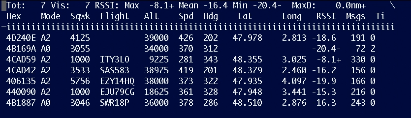
Killing the process shows statistics:

It's fascinating that the information is public.

Ingest into a time-series database​

By default, we stream the latest airplane positions in JSON. If we would like to collect the data for analysis and visualization, then we'll need to store the data over time. For that, we'll need a time-series database.

If you're using the base QuestDB RPi server server, great! Proceed.

If not, you can use any QuestDB instance, whether hosted on your own laptop, in AWS or Azure, or in QuestDB Cloud. Ensure QuestB is running before you continue. Check the QuestDB quick start for help. Open source!

Why QuestDB?​

QuestDB is a high-performance time-series database. It's a great fit for time-series data, such as that generated by sensor-based or IoT usecases.

Given airplanes do everything relative to the bounds of time, a specialized time-series database is a natural fit. And QuestDB can handle millions of incoming rows per second, even on modest hardware.

But getting data in at high speeds is half the battle. It needs to be organized, too! QuestDB handles "out-of-order" indexing, ensuring that data is indexed in-time. Deduplication also functions on in-bound data, ushering clean data into the database even at very high scale.

With clean data, we can perform interesting analysis via SQL queries or setup dashboards for real-time visualizations. More on that later!

Back to building -->

Small Python script​

The json file we need to ingest into QuestDB looks like the following:

{ "now" : 1712248732.7,
  "messages" : 27549,
  "aircraft" : [
    {"hex":"3985a6","flight":"AFR47DW ","alt_baro":27375,"ias":290,"mach":0.732,"mag_heading":322.9,"baro_rate":-2848,"geom_rate":-2912,"squawk":"10>
    {"hex":"4b17f8","alt_baro":38000,"ias":237,"mach":0.752,"mag_heading":319.2,"baro_rate":-32,"geom_rate":-32,"nav_qnh":1012.8,"nav_altitude_mcp":>
    {"hex":"3946e1","version":0,"mlat":[],"tisb":[],"messages":20,"seen":102.5,"rssi":-17.5},
    {"hex":"39b40a","mlat":[],"tisb":[],"messages":16,"seen":78.3,"rssi":-18.6},
    {"hex":"398477","flight":"SVW21DX ","alt_baro":41000,"alt_geom":41075,"gs":407.5,"ias":229,"tas":434,"mach":0.776,"track":205.7,"roll":-0.2,"mag>
    {"hex":"4ca90a","flight":"ITY325  ","alt_baro":26000,"alt_geom":26425,"gs":480.1,"ias":308,"tas":450,"mach":0.748,"track":146.6,"track_rate":0.0>
    {"hex":"4853d0","flight":"TRA15F  ","alt_baro":41000,"alt_geom":41100,"gs":422.3,"ias":232,"tas":438,"mach":0.784,"track":194.4,"track_rate":-0.>
    {"hex":"400f02","flight":"EZY32JU ","alt_baro":37975,"alt_geom":38250,"gs":369.0,"ias":242,"tas":428,"mach":0.764,"track":332.7,"track_rate":-0.>
    {"hex":"4079f7","flight":"BAW14R  ","alt_baro":29000,"alt_geom":29400,"gs":468.7,"ias":268,"tas":412,"mach":0.696,"track":93.2,"track_rate":0.00>
    {"hex":"3c6584","flight":"DLH31K  ","alt_baro":38000,"alt_geom":38175,"gs":497.1,"ias":248,"tas":442,"mach":0.784,"track":66.5,"track_rate":0.00>
    {"hex":"4d23ea","category":"A3","version":0,"mlat":[],"tisb":[],"messages":37,"seen":127.6,"rssi":-17.5},
    {"hex":"406a93","flight":"EZY74VN ","alt_baro":35000,"alt_geom":35375,"gs":467.2,"ias":243,"tas":412,"mach":0.724,"track":143.2,"track_rate":0.2>
    {"hex":"3944e5","alt_baro":27250,"alt_geom":26800,"gs":413.7,"ias":269,"mach":0.668,"track":162.7,"mag_heading":169.3,"baro_rate":2176,"geom_rat>
    {"hex":"3964f8","version":2,"sil_type":"perhour","mlat":[],"tisb":[],"messages":129,"seen":112.0,"rssi":-17.2},
    {"hex":"4866de","flight":"TRA24K  ","alt_baro":37000,"alt_geom":37375,"gs":422.6,"ias":253,"tas":440,"mach":0.784,"track":195.1,"track_rate":0.0>
    {"hex":"43c7ab","flight":"RRR7000 ","alt_baro":43025,"squawk":"5702","mlat":[],"tisb":[],"messages":3368,"seen":0.1,"rssi":-15.6},
    {"hex":"440864","flight":"GAC267Q ","alt_baro":26000,"alt_geom":26400,"gs":339.0,"ias":207,"tas":308,"mach":0.512,"track":156.5,"roll":0.0,"mag_>
    {"hex":"406a95","gs":508.8,"track":113.4,"baro_rate":0,"category":"A3","version":2,"nac_v":1,"sil_type":"perhour","mlat":[],"tisb":[],"messages">
    {"hex":"3c49b6","alt_baro":36000,"version":2,"sil_type":"perhour","mlat":[],"tisb":[],"messages":392,"seen":31.6,"rssi":-18.3},
    {"hex":"4d2500","category":"A3","version":2,"sil_type":"perhour","mlat":[],"tisb":[],"messages":376,"seen":78.0,"rssi":-17.1},
    {"hex":"02006e","version":2,"sil_type":"perhour","mlat":[],"tisb":[],"messages":219,"seen":102.9,"rssi":-17.3},
    {"hex":"43eada","alt_baro":38775,"version":2,"sil_type":"perhour","mlat":[],"tisb":[],"messages":167,"seen":26.2,"rssi":-17.7},
    {"hex":"440090","version":0,"mlat":[],"tisb":[],"messages":9,"seen":209.7,"rssi":-17.6},
    {"hex":"342059","flight":"FIN08PL ","alt_baro":34975,"alt_geom":35325,"gs":427.3,"ias":266,"tas":448,"mach":0.784,"track":203.4,"track_rate":-0.>
  ]
}

The JSON can be updated at a custom interval using the argument write-json-every when launching dump1090. It default to every 1 second. The object contains an identifier, altitude, coordinates, speed, flight number, and more.

To ingest this data into QuestDB, we'll use the Questdb Python client. But you can use any client or ingest method that you wish.

Using Python, we'll apply a small script. This script assumes that the QuestDB server is in the same location as the Raspberry Pi with the additional components. That means if you're using the same Raspberry Pi from the server article, you'd use localhost:9000 and run this script as we demonstrate.

Apart from that, there is nothing too mystifying, other than that we check for the presence of all important keys before sending the data. In other words, we discard incomplete readings:

from questdb.ingress import Sender, TimestampNanos
import json
from time import sleep

file = '/home/tanc/aircraft/aircraft.json'
conf = f'http::addr=localhost:9000;'

def readData(file):
        f=open(file)
        data=json.load(f)
        f.close()
        return data

def parseData(data):
        for f in data['aircraft']:
                if all(k in f.keys() for k in ('lat','lon','ias','flight','alt_baro','track')):
                        with Sender.from_conf(conf) as sender:
                                sender.row(
                                'aircraft',
                                symbols={},
                                columns={'lat': f['lat'],
                                        'lon': f['lon'],
                                        'ias': f['ias'],
                                        'flight':f['flight'],
                                        'alt_baro':f['alt_baro'],
                                        'track':f['track']},
                                at=TimestampNanos.now())
                                sender.flush()

while True:
        data = readData(file)
        parseData(data)
        sleep(0.5)

With a running QuestDB server, a running dump1090, and the above script, we can see data arriving into our QuestDB database:

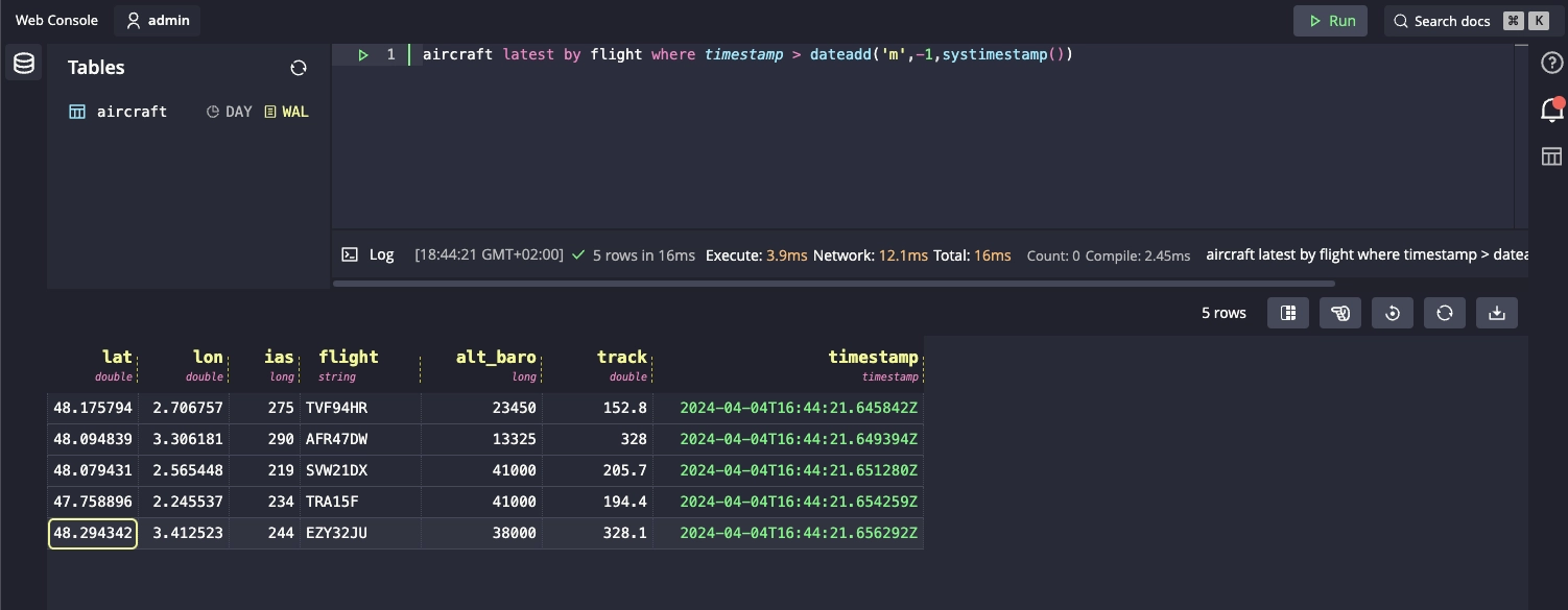
Neat!

Build your own radar​

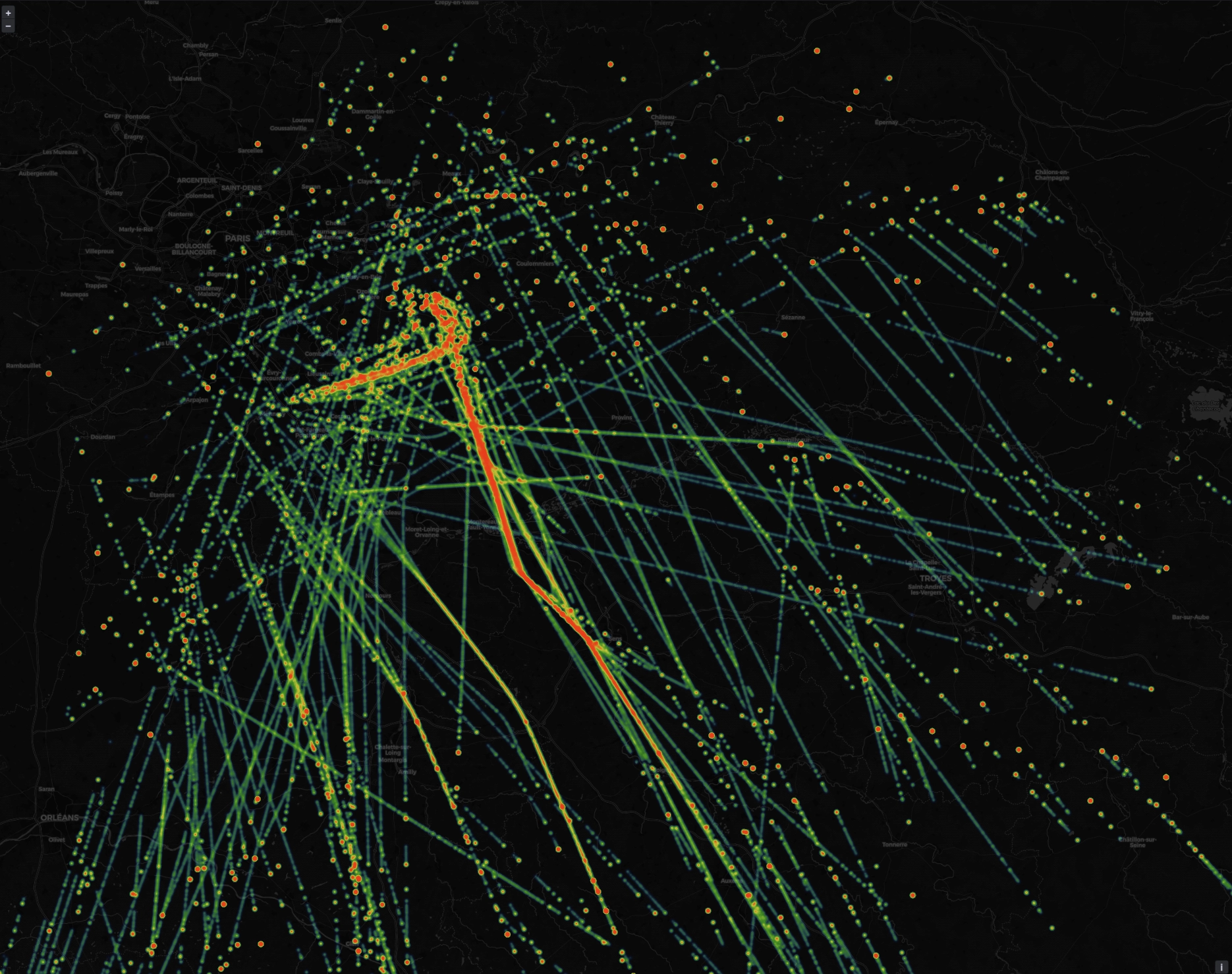
A stream of data has arrived into QuestDB. Nice. But capturing the events is only one step.

Time to have some fun and build our own radar server. With it, we can visualize our flight data in real-time, however we please.

First, let's install and start Grafana:

sudo mkdir -p /etc/apt/keyrings/
wget -q -O - https://apt.grafana.com/gpg.key | gpg --dearmor | sudo tee /etc/apt/keyrings/grafana.gpg > /dev/null
echo "deb [signed-by=/etc/apt/keyrings/grafana.gpg] https://apt.grafana.com stable main" | sudo tee /etc/apt/sources.list.d/grafana.list
sudo apt-get update
sudo apt-get install -y grafana
sudo /bin/systemctl enable grafana-server
sudo /bin/systemctl start grafana-server

With QuestDB and Grafana running, we setup our radar.

But before that, one thing we should do is increase the refresh rate frequency of Grafana from the default 5s so that the charts update continuously. This will give our charts a fluid, real-time feeling. 1 second or less is a great bet.

We can then create a GeoMap panel and populate it with a query such as the following:

SELECT
  timestamp,
  flight,
  alt_baro,
  track,
  ias,
  lat,
  lon
FROM
  aircraft
LATEST BY
  flight
WHERE
  $__timeFilter(timestamp)

This query uses the LATEST BY keyword which shows us the last record for each unique flight in the target time interval.

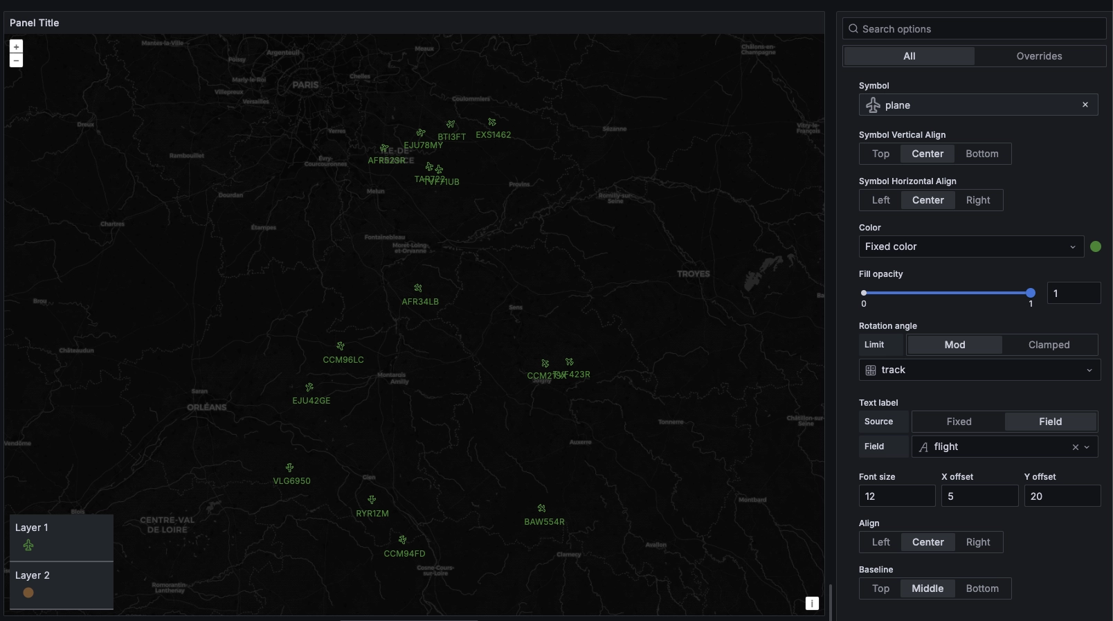
One nice feature of the GeoMap panel is that we can orient symbols based on their bearing. Our map looks like so, with the corresponding settings on the right hand side:

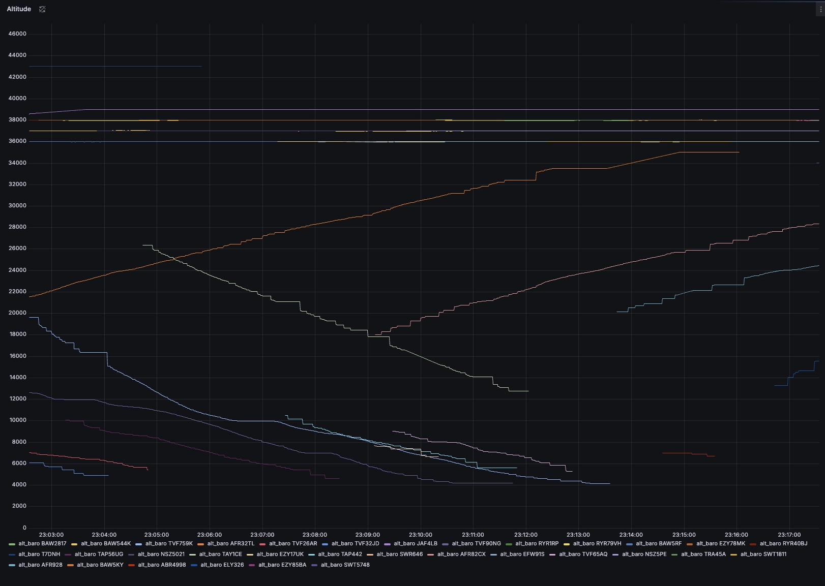
We can also get some situational awareness in terms of altitude with a simple query:

SELECT
  timestamp,
  flight,
  alt_baro
FROM
  aircraft
WHERE
  $__timeFilter(timestamp)

The result shows us both the altitude over time, and the limits of our ground station. We lose detection below a certain altitude floor around 5,000 feet, probably because of lack of line of sight!

Going further with Grafana​

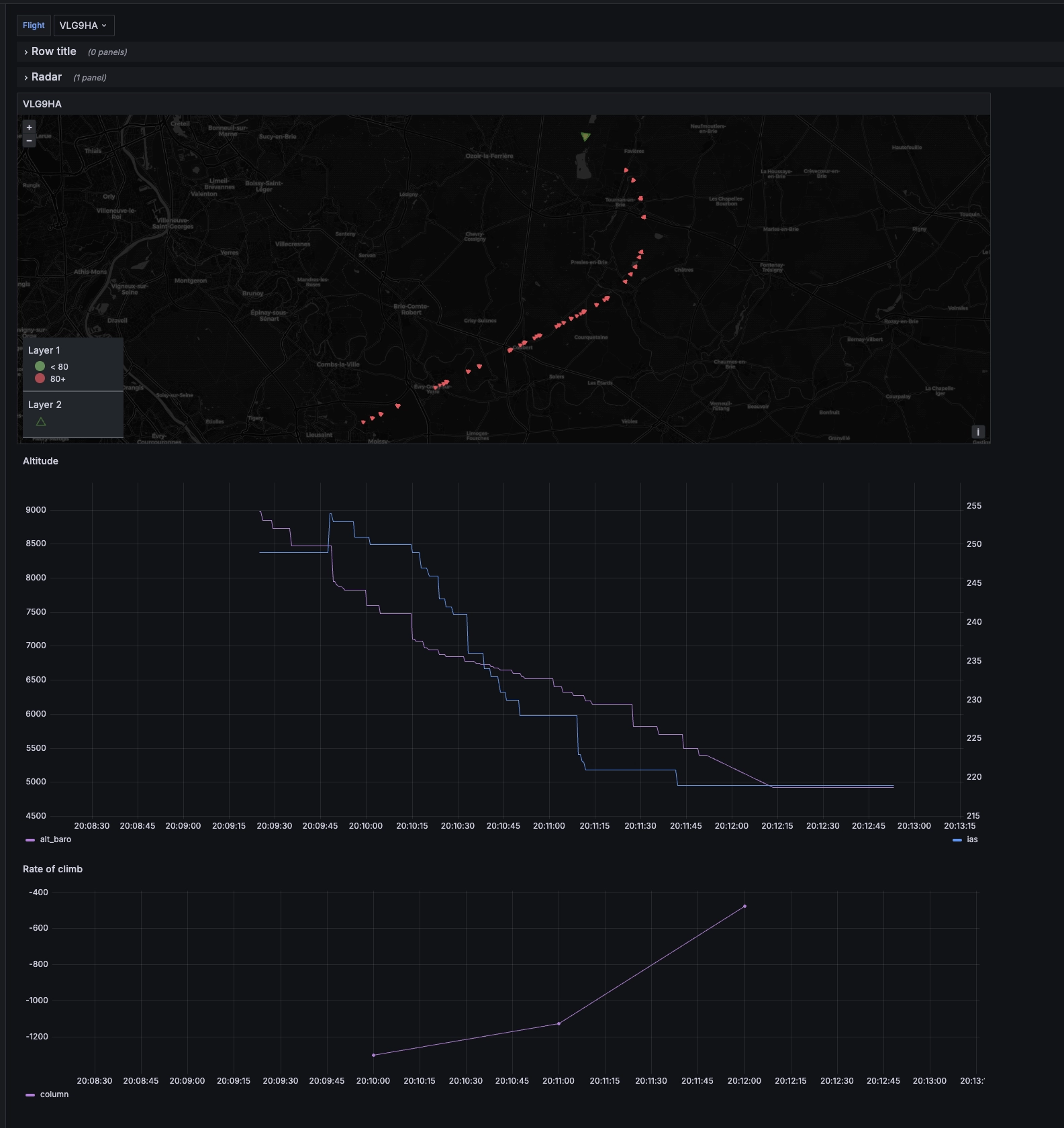
We can use Grafana variables to isolate single flights. From there, we can look at the flight's recent position on a map alongside other statistics such as its altitude and speed. This tells a three-dimensional story:

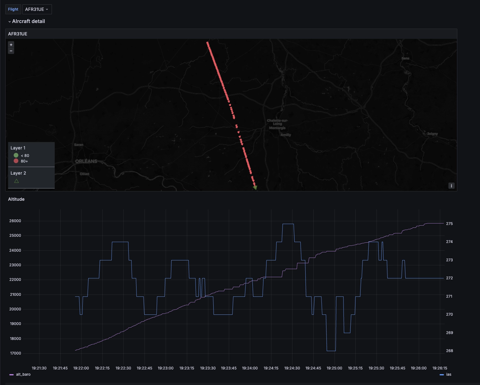
For example, this flight is climbing at a target speed of around 270 Knots Indicated Airspeed (KIAS):

SELECT
  timestamp,
  alt_baro
FROM
  aircraft
WHERE
  flight = '$Flight'
  AND $__timeFilter(timestamp)

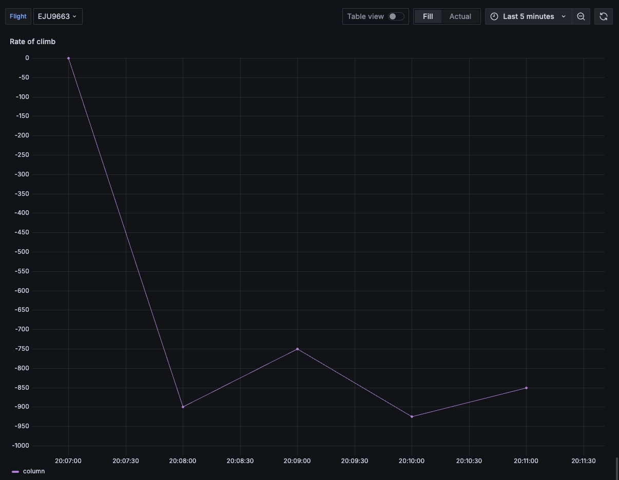
We can also look at other derivatives such as rate of climb. For example, we can use LT JOIN to compare the current altitude to the previous one, and then smoothe the results with a SAMPLE BY.

WITH
  x AS (
    SELECT
      timestamp,
      LAST(alt_baro) AS alt
    FROM
      aircraft
    WHERE
      flight = '$Flight'
      AND $__timeFilter(timestamp)
    SAMPLE BY
      1m ALIGN TO CALENDAR
  ),
  y AS (
    SELECT
      timestamp,
      LAST(alt_baro) AS alt
    FROM
      aircraft
    WHERE
      flight = '$Flight'
      AND $__timeFilter(timestamp)
    SAMPLE BY
      1m ALIGN TO CALENDAR
  )
SELECT
  x.timestamp,
  x.alt - y.alt
FROM
  x
  LEFT JOIN
  y

The result indeed gives us an indication of the rate of climb over time:

We can now enjoy looking at our new dashboard.

Looks like VLG9HA is about to land, safe and sound!

Eager for another project?

Checkout our tutorial other Raspberry Pi tutorial:

• Build a temperature IoT sensor with Raspberry Pi Pico & QuestDB

What else is cool about QuestDB?​

QuestDB is a high-performance time-series database. It's great for hobby projects, and also for capturing hyper-streams of data seen in:

• rockets bound for outer-space
• nuclear reactors
• the cranes moving our goods at the worlds busiest ports
• the fastest cars ripping around the track in the Formula 1

Once inside, the analysis, visualization and querying of that data is paramount. QuestDB - as a time-series native database - has very useful SQL extensions to manipulate time-based data:

• SAMPLE BY summarizes data into chunks based on a specified time interval, from a year to a microsecond
• WHERE IN to compress time ranges into concise intervals
• LATEST ON for latest values within multiple series within a table
• ASOF JOIN to associate timestamps between a series based on proximity; no extra indices required

SQL is known to many, and our documentation can get you comfortable quickly, if you're unfamiliar.

For these reasons and more, QuestDB is an excellent fit for your IoT cases.

We hope you like it!