QuestDB 6.2, our previous minor version release, introduced JIT (Just-in-Time) compiler for SQL filters. As we mentioned last time, the next step would be to parallelize the query execution when suitable to improve the execution time even further and that's what we're going to discuss and benchmark today. QuestDB 6.3 enables JIT compiled filters by default and, what's even more noticeable, includes parallel SQL filter execution optimization allowing us to reduce both cold and hot query execution times quite dramatically.
Prior to diving into the implementation details and running some before/after benchmarks for QuestDB, we'll be having a friendly competition with two popular time series and analytical databases, TimescaleDB and ClickHouse. The purpose of the competition is nothing more but an attempt to understand whether our parallel filter execution is worth the hassle or not.
Comparing with other databases
Our test box is a c5a.12xlarge AWS VM running Ubuntu Server 20.04 64-bit. In practice, this means 48 vCPU and 96 GB RAM. The attached storage is a 1 TB gp3 volume configured for 1,000 MB/s throughput and 16,000 IOPS. Apart from that, we'll be using QuestDB 6.3.1 with the default settings which means both parallel filter execution and JIT compilation being enabled.
In order to make the benchmark easily reproducible, we're going to use TSBS benchmark utilities to generate the data. We'll be using so-called IoT use case:
./tsbs_generate_data --use-case="iot" \
                     --seed=123 \
                     --scale=5000 \
                     --timestamp-start="2020-01-01T00:00:00Z" \
                     --timestamp-end="2020-07-01T00:00:00Z" \
                     --log-interval="60s" \
                     --format="influx" > /tmp/data \
                     /
The above command generates six months of per-minute measurements for 5,000
truck IoT devices. This yields almost 1.2 billion records stored in a table
named readings.
Loading the data is as simple as:
./tsbs_load_questdb --file /tmp/data
Now, when we have the data in the database, we're going to execute the following
query on the readings table:
SELECT *
FROM readings WHERE velocity > 90.0
 AND latitude >= 7.75 AND latitude <= 7.80
 AND longitude >= 14.90 AND longitude <= 14.95;
This (kinda synthetic) query aims to find all measurements sent from fast-moving trucks in the given location. Apart from that, it has a filter on three DOUBLE columns and doesn't include analytical clauses, like GROUP BY or SAMPLE BY, which is exactly what we need.
Our first competitor is TimescaleDB 2.6.0 running on top of PostgreSQL 14.2. As
the official installation guide suggests, we made sure to run timescaledb-tune
to fine-tune TimescaleDB for better performance.
We generate the test data with the following command:
./tsbs_generate_data --use-case="iot" \
                     --seed=123 \
                     --scale=5000 \
                     --timestamp-start="2020-01-01T00:00:00Z" \
                     --timestamp-end="2020-07-01T00:00:00Z" \
                     --log-interval="60s" \
                     --format="timescaledb" > /tmp/data \
                     /
That's the same command as before, but with the format argument set to
timescaledb. Next, we load the data:
./tsbs_load_timescaledb --pass your_pwd --file /tmp/data
Be prepared to wait for quite a while for the data to get in this time. We observed 5-8x ingestion rate difference between QuestDB and two other databases in this particular environment. Yet, that's nothing more but a note for anyone who wants to repeat the benchmark. If you'd like learn more on the ingestion performance topic, check out this blog post.
Finally, we're able to run the first query and measure the hot execution time. Yet, if we do it, it would take more than 15 minutes for TimescaleDB to execute this query. At this point, experienced TimescaleDB & PostgreSQL users may suggest us to add an index to speed up this concrete query. So, let's do that:
CREATE INDEX ON readings (velocity, latitude, longitude);
With an index in place, TimescaleDB can execute the query much much faster, in around 4.4 seconds. To get the full picture, let's include one more contestant.
The third member of our competition is ClickHouse 22.4.1.752. Just like with
TimescaleDB, the command to generate the data stays the same with only the
format argument being set to clickhouse. Once the data is generated, it can
be loaded into the database:
./tsbs_load_clickhouse --file /tmp/data
We're ready to do the benchmark run.
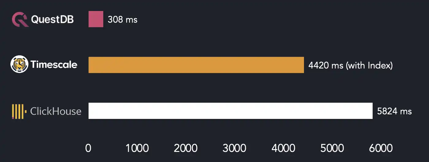
The above chart shows that QuestDB is an order of magnitude faster than both TimescaleDB and ClickHouse in this specific query.
Interestingly, an index-based scan doesn't help TimescaleDB to win the competition. This is a nice illustration of the fact that a specialized parallelism-friendly storage model may save you from having to deal with indexes and paying the additional overhead during data ingestion.
As the next step, let's give another popular type of query a go. In the world of time series data, it's common to query only the latest rows based on a certain filter. QuestDB supports that elegantly through negative LIMIT clause values. If we were to query ten latest measurements sent from fast-moving, yet fuel-efficient trucks it would look like the following:
SELECT *
FROM readings
WHERE velocity > 75.0 AND fuel_consumption < 10.0
LIMIT -10;
Notice the LIMIT -10 clause in our query. It basically asks the database to return the last 10 rows that correspond to the filter. Thanks to the implicit ascending order based on the designated timestamp column, we also didn't have to specify ORDER BY clause.
In TimescaleDB this query would look more verbose:
SELECT *
FROM readings
WHERE velocity > 75.0 AND fuel_consumption < 10.0
ORDER BY time DESC
LIMIT 10;
Here, we had to specify descending ORDER BY and LIMIT clauses. When it comes to
ClickHouse, the query would look just like for TimescaleDB with the exception of
another column being used to store timestamps (created_at instead of time).
How do databases from our list deal with such query? Let's measure and find out!
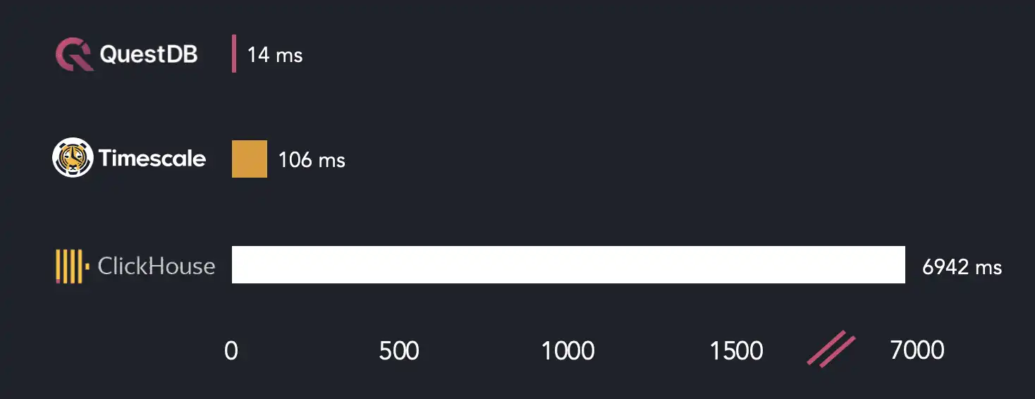
This time, surprisingly or not, TimescaleDB does a better job than ClickHouse.
That's because, just like QuestDB, TimescaleDB filters the data starting with
the latest time-based partitions and stops the filtering once enough rows are
found. We could also add an index on the velocity and fuel_consumption
columns, but it won't change the result. That's because TimescaleDB doesn't use
the index and does a full scan instead for this query. Thanks to such behavior,
both QuestDB and TimescaleDB are significantly faster than ClickHouse in the
exercise.
Needless to say, that both TimescaleDB and ClickHouse are great pieces of engineering. Your mileage may vary and performance of your particular application depends on a large number of factors. So, as with any benchmark, take our results with a grain of salt and make sure to measure things on your own.
That should be it for our comparison and now it's time to discuss the design decisions behind our parallel SQL filter execution.
How does it work?
First, let's quickly recap on QuestDB's storage model to understand why it supports efficient multi-core execution. The database has a column-based append-only storage model. Data is stored in tables, with each column stored in its own file or multiple files in case when the table is partitioned by the designated timestamp.
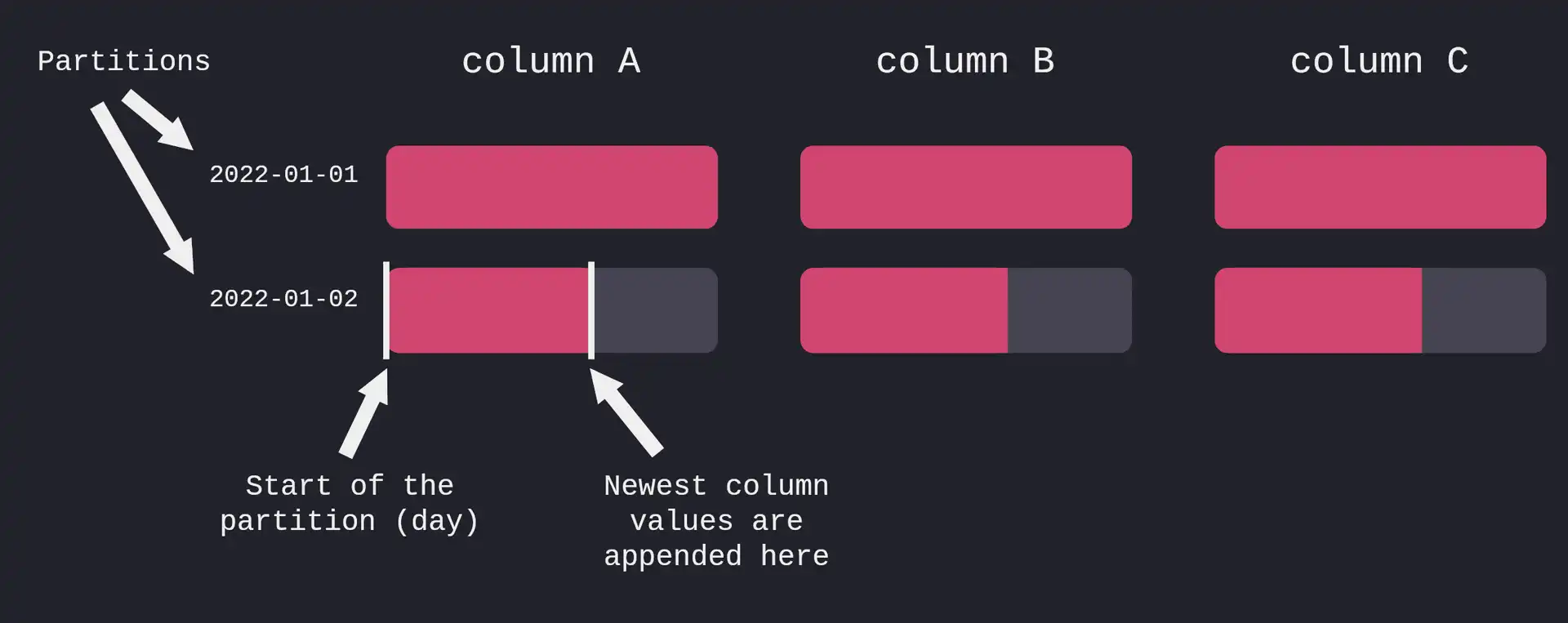
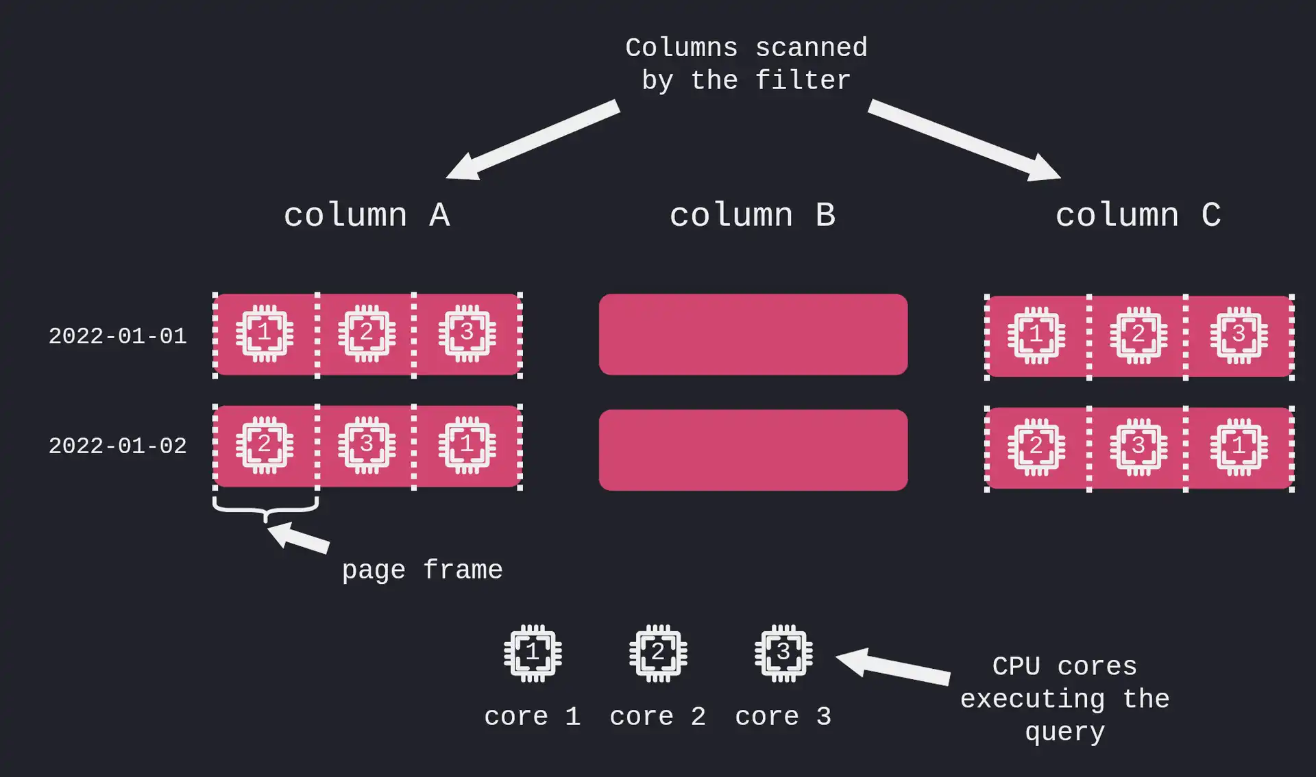
When a SQL filter (think, WHERE clause) is executed, the database needs to scan the files for the corresponding filtered columns. As you may have already guessed, when the column files are large enough, or the query touches multiple partitions, filtering the records on a single thread is inefficient. Instead, the file(s) could be split into contiguous chunks (we call them "page frames"). Then, multiple threads could execute the filter on each page frame utilizing both CPU and disk resources in a much more optimal way.
We already had this optimization in place for some of the analytical types of queries, but not for full or partial table scan with a filter. So, that's basically what we've added in version 6.3.
As usual, there are edge cases and hidden reefs, so the implementation is not as simple as it may sound. Say, what if your query has a filter and a LIMIT -10 clause, just like in our recent benchmark? Then the database should execute the query in parallel, fetch the last 10 records and cancel the remaining page frame filtering tasks, so that there is no useless filtering done by other worker threads. A similar cancellation should take place in the face of a closed PG Wire or HTTP connection or a query execution timeout. So, as you already saw in the above comparison, we made sure to handle all of these edge cases. If you're interested in the implementation details, go check this lengthy pull request.
From the end user perspective, this optimization is always enabled and applies to non-JIT and JIT-compiled filters. But how does it improve QuestDB's performance? Let's find out!
Speed up measurements
We'll be using the same benchmark environment as above while using a slightly different query to keep things simple:
SELECT count(*)
FROM readings
WHERE velocity > 75.0 AND fuel_consumption < 10.0;
This query counts the total number of measurements sent from fast-moving, yet fuel-efficient trucks.
First, we focus on cold execution time, i.e. situation when the column files data is not in the OS page cache. Multi-threaded runs use QuestDB 6.3.1 while single-threaded ones use 6.2.0 version of the database. That's because JIT compilation is only available in when parallel filter execution is on starting from 6.3. The database configuration is kept default, except for the JIT being disabled or enabled in the corresponding measurements. Also notice while this given query supports JIT compilation, there is a number of limitations for the types of the queries supported by the JIT compiler.
The below chart shows the cold execution times.
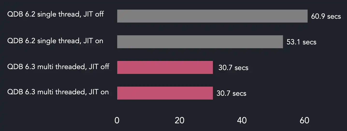
What's that? Parallel filter execution is only two times faster. More than that, enabled JIT-compiled filters have almost no effect on the end result. The thing is that the disk is the bottleneck here.
Let's try to make some sense out of these results. It takes around 30.7 seconds for QuestDB 6.3 to execute the query when the data is only on disk. The query engine has to scan two groups of column files, 182 partitions each having two 50 MB files. This gives us around 18.2 GB of on-disk data and around 592 MB/s disk read rate. That's lower than the configured maximum in our EBS volume, but we should keep in mind allowed 10% fluctuations from the maximum throughput and, what's even more important, individual limits for EBS-optimized instances. Our instance type is c5a.12xlarge and, according to the AWS documentation, it's limited with 594 MB/s on 128 KiB I/O which is very close to our back of the envelope calculation.
Long story short, we're maxing out the disk with multi-threaded query execution while single-threaded execution time in version 6.2 stays the same. With this in mind, further instance type and volume improvements would lead to better performance.
Things should get even more exciting when it comes to hot execution scenario, so there we go. In the next and all of the subsequent benchmark runs, we measure the average hot execution time for the same query.
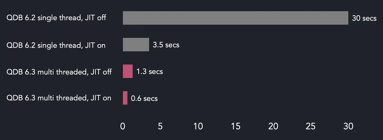
On this particular box, default QuestDB configuration leads to 16 threads being used for the shared worker pool. So, both 6.3 runs execute the filter on multiple threads speeding up the query when compared with the 6.2 runs. Another observation is almost 1x difference between JIT-compiled and non-JIT filters on 6.3. So, even with many cores available to parallel query execution, it's a good idea to keep JIT compilation enabled.
You might have noticed a weird proportion in the above chart. Namely, the difference between the execution times when JIT compilation is disabled. QuestDB 6.2 takes 30 seconds to finish the query with a single thread, while it takes only roughly 1.3 seconds on 6.3. That's 23x improvement and it's impossible to explain it only with parallel processing (remember, we run the filter on 16 threads). So, what may be the reason?
The thing is that parallel filter execution uses the same batch-based model as
JIT-compiled filter functions. This means that the filter is executed in a
tight, CPU-friendly loop while the resulting identifiers for the matching rows
are stored in an intermediate array. For instance, if we restrict parallel
filter engine to run on a single thread which is as simple as adding
shared.worker.count=1 database setting, the query under test would execute in
around 13.5 seconds. Thus, in this very scenario batch-based filter processing
done on a single thread allows us to cut down 55% of the query execution time.
Obviously, multiple threads available to the engine let it run even faster.
Refer to this
blog post
for more information on how we do batch-based filter processing in our SQL JIT
compiler.
There is one more optimization opportunity around the query we used here.
Namely, in case of queries that select only simple aggregate functions, like
count(*) or max(*), and no column values we could push down the functions
into the filter loop. As an example, the filter loop will be incrementing the
count(*) function's counter in-place rather than doing a more generic
accumulation of the filtered row identifiers. You could say that such queries
are rather niche, but they could be met in various dashboard applications. Thus,
it's something that we definitely consider adding in future.
What's next?
Certainly, parallel SQL filter execution introduced in 6.3 is not the final point in our quest. As we've mentioned already, we have multi-threading in place for aggregate queries, like SAMPLE BY or GROUP BY, but only for certain shapes of them. Aggregate functions push-down is another potential optimization. So stay tuned for further improvements!
As always, we encourage our users to try out 6.3.1 release on your QuestDB instances and provide feedback in our Slack Community. You can also play with our live demo to see how fast it executes your queries. And, of course, open-source contributions to our project on GitHub are more than welcome.